
Module 4: Responsible Data Storytelling
Gestalt’s Principles
In the 1900s, the Gestalt School of Psychology defined some basic principals of visual perception that are still widely accepted today and can be applied as a framework in developing data visualizations.
Proximity
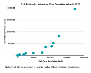
Proximity refers to the closeness of visual elements. The separate design entities come together to create a “unified whole” due to their distance/space from one another. The closer the entities appear, the stronger the relationship. See Figure 4.1[1] below for an example of how proximity in a scatterplot defines a relationship.
Similarity
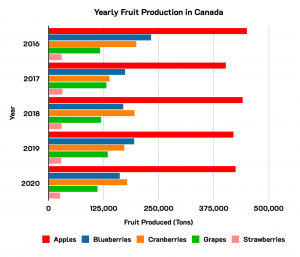
Similarity refers to unity and wholeness (e.g. shapes, text, colours). Elements that look alike are seen as belonging to the same group or creating a pattern to form a singular unit. See Figure 4.2[2] for an example of how repeating colours represent similarity.
Continuity
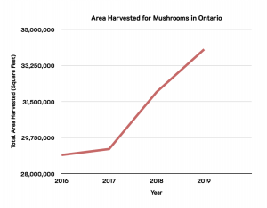
Continuity refers to our eyes continuing the design of a path, line, or curve , though it may extend beyond the page. The mind will automatically fill in the gap to “go with the flow”. See Figure 4.3[3] for an example of continuity.
Closure
Closure refers to our mind completing missing portions of a design. There must be enough parts available for the image to be “filled in”; if the image is too abstract, there are minimal reference points for the mind to complete it. See Figure 4.4[4] for an example of how our mind automatically imagine a line connecting the 2 broken ones.
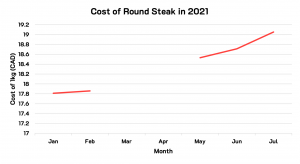
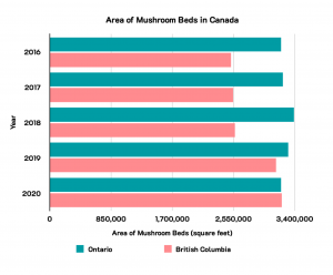
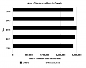
Figure-Ground
Figure-Ground refers to the design’s focal point (figure) and background (ground) details. Using figure-ground will allow the audience to automatically find the areas to focus upon. Figure 4.4[5] displays good contrast, whereas Figure 4.5 displays poor contrast with the same data.
- Statistics Canada. Table 32-10-0364-01 Area, production and farm gate value of marketed fruits. Data is reproduced and distributed on an "as is" basis with the permission of Statistics Canada. Retrieved January 9th, 2022. DOI: https://doi.org/10.25318/3210036401-eng. Statistics Canada Open Licence: https://www.statcan.gc.ca/en/reference/licence ↵
- Statistics Canada. Table 32-10-0364-01 Area, production and farm gate value of marketed fruits. Data is reproduced and distributed on an "as is" basis with the permission of Statistics Canada. Retrieved January 9th, 2022. DOI: https://doi.org/10.25318/3210036401-eng. Statistics Canada Open Licence: https://www.statcan.gc.ca/en/reference/licence ↵
- Statistics Canada. Table 32-10-0356-01 Area, production and sales of mushrooms. Data is reproduced and distributed on an "as is" basis with the permission of Statistics Canada. Retrieved January 8th, 2022. DOI: https://doi.org/10.25318/3210035601-eng. Statistics Canada Open Licence: https://www.statcan.gc.ca/en/reference/licence ↵
- Statistics Canada. Table 18-10-0002-01 Monthly average retail prices for food and other selected products. Data is reproduced and distributed on an "as is" basis with the permission of Statistics Canada. Retrieved February 2nd, 2022. DOI: https://doi.org/10.25318/1810000201-eng. Statistics Canada Open Licence: https://www.statcan.gc.ca/en/reference/licence ↵
- Statistics Canada. Table 32-10-0356-01 Area, production and sales of mushrooms. Data is reproduced and distributed on an "as is" basis with the permission of Statistics Canada. Retrieved January 8th, 2022. DOI: https://doi.org/10.25318/3210035601-eng. Statistics Canada Open Licence: https://www.statcan.gc.ca/en/reference/licence ↵
