8.5 The Effect of an additional Zero on the 2nd Order System Response

To make matters even more complicated, while the shapes of transients depend on the pole locations, zeros of the transfer function decide the magnitude of each component and thus also have an effect on the system response. In Chapter 8.2 we learned that the magnitude of a particular transient component can be very small and thus insignificant if a zero is near that pole location – a pole-zero near cancellation. When that is not the case, the effect of a zero may be significant, depending on its location. Let’s assume that a standard second order system has an additional zero at s = -a. The transfer function gain is adjusted to remain constant:

The transfer function in Equation 8‑2 can be considered as a sum of two components – the first component is the standard second order model, but the second component has a derivative term in it – a zero is basically an s-operator and as such it acts as a derivative on the response signal.

Now consider its effect on the system response [latex]Y(s)[/latex] to a unit step:

[latex]Y(s) = G_{mod}(s) \cdot R(s) = G_{mod}(s) \cdot \frac{1}{s}[/latex]

[latex]Y(s) = \Bigg\{  K_{dc} \cdot \frac{ \omega_{n}^{2}}{s(s^{2}+2\zeta\omega_{n} + \omega_{n}^{2})} \Bigg\} + \frac{1}{a} s\Bigg\{  K_{dc} \cdot \frac{ \omega_{n}^{2}}{s(s^{2}+2\zeta\omega_{n} + \omega_{n}^{2})} \Bigg\}[/latex]

The above expression for the system response is again a superposition of two components: a step response of the standard second order model, and a derivative of the same step response, but with a multiplier 1/a. Depending on the magnitude of a, this component may be small or large. Thus, if a is large, i.e. the zero is far away in the LHP, the magnitude of this derivative term is insignificant and can be safely ignored. However, if the zero is placed in the significant region close to the Imaginary axis, the magnitude of this signal component rapidly increases. The superposition of a signal and its derivative creates a large “hump” in the system response, in essence an exaggerated Percent Overshoot.

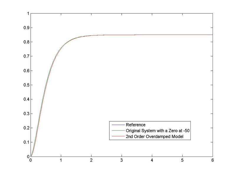
As an example, consider a second order overdamped system with poles at -5 and -3, and an additional zero at a = -50

[latex]G(s) = 0.85 \cdot \frac{15}{(s+5)(s+3)} \cdot \frac{(s+50)}{50} = \frac{0.255s + 12.75}{s^{2} + 8s+15}[/latex]

The plot of its step response is shown in Figure 8‑8, compared to the response of a system without the zero added. Again predictably, based on Equation 8‑2 there is virtually no effect of the zero far in the insignificant region on the system response, with the original system (i.e. the one with the zero) ever so slightly faster. If we were looking for a simpler model for this system, the zero can safely be ignored:

[latex]G_{mod}(s) = 0.85 \cdot \frac{15}{s^{2} + 8s + 15}[/latex]

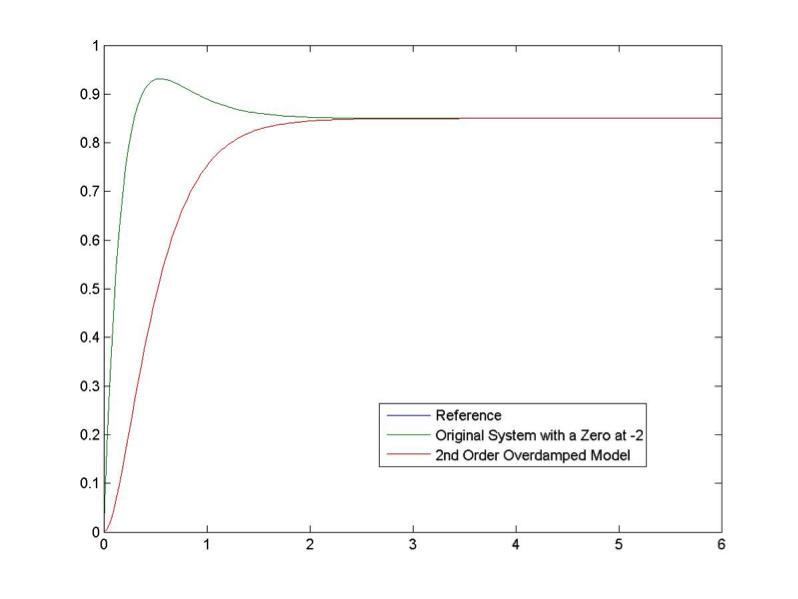
Now, let’s see what happens when the zero is moved into the significant region close to the dominant poles, as shown in Figure 8‑9 . Assume a = -2:

[latex]G(s) = 0.85 \cdot \frac{15}{(s+5)(s+3)} \cdot \frac{(s+2)}{2} = \frac{6.37s + 12.75}{s^{2} + 8s+15}[/latex]

Notice that the settling time again is not affected. Conclusion – the presence of a zero in the significant region in the LHP (i.e. where the dominant poles of the system are), has a derivative effect on the system response. That derivative effect results in a faster response but with an increased Overshoot. We would not be able to replace the system dynamic with a simplified model – the zero has to be included in the system description.

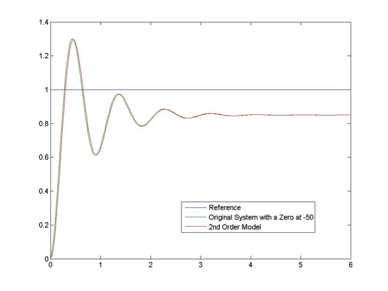
Next, consider a second order system with a pair of complex poles is: [latex]s_{1} = -1.4+j6.86, s_{12} = -1.4 - j6.86[/latex] and an additional zero at a = -50, as shown in Figure 8‑10, compared to the response of a system without the zero added.

[latex]G(s) = 0.85 \cdot \frac{49}{s^{2}+2.8s + 49} \cdot \frac{(s+50)}{50} = \frac{0.833s + 41.7}{s^{2} + 2.8s+49}[/latex]

Predictably, based on Equation 8‑2 there is virtually no effect of the zero far in the insignificant region on the system response, with the original system (i.e. the one with the zero) ever so slightly faster. If we were looking for a simpler model for this system, the zero can safely be ignored.

[latex]G(s) = 0.85 \cdot \frac{49}{s^{2}+2.8s + 49}[/latex]

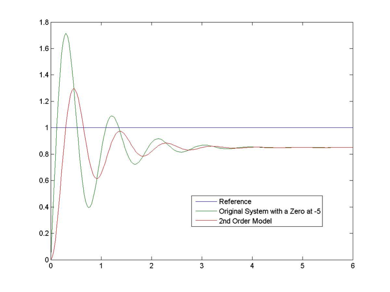
Now, let’s see what happens when the zero is moved into the significant region close to the dominant poles. Assume a =-5. Plots are shown in Figure 8‑11.

[latex]G(s) = 0.85 \cdot \frac{49}{s^{2}+2.8s + 49} \cdot \frac{(s+50)}{50} = \frac{0.833s + 41.7}{s^{2} + 2.8s+49}[/latex]

As in the case of an overdamped system, the magnitude of the derivative term in Equation 8‑2 is much larger now. As a result, the system response is much faster (shorter Rise Time), while the Percent Overshoot is much worse (larger). The frequency of oscillations and Settling Time are not affected. We would not be able to replace the system dynamic with a simplified model – the zero has to be included in the description.