8.2 Minimum Realizations and Reduced Order Models – Part 1

Consider a certain process described by a block diagram below, where:

[latex]G_{1}(s)=\frac{10(s+1.05)}{(s+3)(s+2}G_{2} = \frac{5(s+3)(s+2)}{(s+58)(s+0.9)}[/latex]

[latex]H_{1}(s) = 1[/latex]

[latex]H_{2}(s) = \frac{1}{s+2}[/latex]

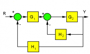
Looking at the dynamics of the transfer functions, this is a 5th order process. Let’s find its transfer function:

[latex]L_{1}-G_{2}H_{2}[/latex]      [latex]L_{2}-G_{2}G_{2}H_{1}[/latex]      [latex]P_{1} = G_{1}G_{2}[/latex]     [latex]\Delta = 1 - (L_{1} + L_{2})[/latex]

[latex]G(s) = \frac{Y(s)}{R(s)} = \frac{G_{1}(s)G_{2}(s)}{1+G_{2}(s)H_{2}(s) + G_{1}(s)G_{2}(s)H_{1}(s)}[/latex]

[latex]G(s) = \frac{Y(s)}{R(s)} = \frac{50s^{4} + 402.5s^{3} + 1168s^{2} + 1440s + 630}{s^{5} + 120.9s^{4} + 933s^{3} + 2672s^{2} + 3282s + 1436}[/latex]

The transfer function can be factored into a ZPK form as follows:

[latex]G(s) = \frac{Y(s)}{R(s)} =\frac{50(s+3)(s+2)^{2}(s+1.05)}{(s+112.8)(s+3)^{2}(s+1.061)}[/latex]

After pole-zero cancellation is performed (you can use MATLAB minreal function) we have:

[latex]G(s) = \frac{50(s+1.05)}{(s+112.8)(s+1.061)}[/latex]

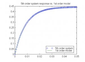
Check the pole-zero map of the system – another near-cancellation is observed between the process pole at s = -1.061 and the zero at s = -1.05. The process response is shown below – it looks exactly like a first order system response, despite 5th order dynamics. Therefore we can build a first order model for this 5th order system:

[latex]G_{model}(s) = \frac{Y(s)}{R(s)} \approx \frac{50}{s+112.8}[/latex]

Note that the multiplier gain K of the system ZPK model should be adjusted so that the model DC gain is the same as the DC gain of the original system:

[latex]K_{dc} = G(0) = \frac{50 \cdot 1.05}{112.8 \cdot 1.061} = 0.4386[/latex]

[latex]K_{dc} = G(0) = \frac{K}{0+112.8} = 0.4386 \rightarrow K = 49.49[/latex]

[latex]G_{model}(s) = \frac{49.5}{s + 112.8}[/latex]

In summary, when system parameters have such values that pole-zero cancellations occur, we can replace the original system transfer function with its so-called minimum realization. In effect, the minimum realization is a model of the system that is of a lower order than the original system, yet, behaves in the same way.

We can also introduce a lower order, or reduced order, model when the pole-zero cancellation is not perfect. Recall that while the zeros of a transfer function do not affect the shape of the system response, they decide values of residues, i.e. magnitudes of each transient component. When a zero is close to a particular pole, the magnitude of the transient associated with that pole will be very small and its contribution to the system response can be ignored, resulting in a reduced order model.

MATLAB minreal function can perform pole-zero cancellations in the system transfer function that may not be immediately obvious. As well, we can use this function to perform near-cancellations where the locations of poles and zeros are not identical but are close. If the cancellation is not perfect, it can be still performed by using the “tol” parameter of the minreal function. If the pole-zero cancellation was not perfect, it is important to make sure that the DC gain of the reduced order model matches the DC gain of the original process.