8.4 The Effect of an Additional Pole on the 2nd Order System Response

In cases where there are more than one or two poles close to the Imaginary axis, a standard second order underdamped model will not be sufficient. The reduced order model may not be possible or it may require an additional real pole or an additional pair of the complex poles. What system response specifications are affected by the presence of an additional real pole? The additional pole will contribute more damping to the system response. This will reduce the Percent Overshoot, but at the same time, it will slow the system response increasing Rise Time and Settling Time. As an example, consider a plot of a step response of an unknown system as shown in Figure 8‑2, and investigate if the standard second order model is appropriate.

At the first glance, the second order model seems appropriate as the system is oscillatory. Let’s read off the PO Settling Time and DC gain of the process: [latex]PO = 33\%, T_{settle(\pm 2\%)} = 3.44[/latex] and [latex]K_{dc} = 0.9[/latex].

We can compute the corresponding damping ratio and then the frequency of natural oscillations:

[latex]\zeta = \sqrt{\frac{\Bigg( -\ln{\bigg(\frac{33}{100}\bigg)}\Bigg)^{2}}{\Bigg(\pi^{2} + \Bigg(-\ln{\bigg(\frac{33}{100}\bigg)} \Bigg)^{2} \Bigg)}} \approx 0.33[/latex]

[latex]3.44 = \frac{4}{0.33\omega_{n}} \rightarrow \omega_{n} = 3.52[/latex]

The resulting model is:

[latex]G_{mod}(s) = 0.9\frac{12.39}{s^{2} + 2.36s + 12.39}=\frac{11.15}{s^{2} + 2.36s + 12.39}[/latex]

Let’s plot the model response in Figure 8‑3, and compare it with the process response:

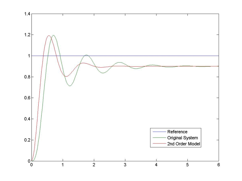
This initial result is quite disappointing. While the Percent Overshoot and the Settling Time seem appropriate, the frequency of oscillations is definitely too low. Let’s adjust to 6 rad/sec, as shown in Figure 8‑4. With the PO and frequency of oscillations reasonably matched, the original system takes longer to settle and it is also visibly lagging in rise time. Let’s try adjusting the damping ratio to 0.17, as shown in Figure 8‑5.

Now, with the frequency of oscillations and the settling time reasonably matched, the model is much more oscillatory – the original system exhibits more damping. The additional damping may be introduced by a real pole that cannot be ignored. The presence of a third pole also slows down the rise time considerably. It is clear now that the second order model is not appropriate here. Let’s assume a 3rd order model with an additional real pole:

Note that in Equation 8‑1 the third pole magnitude a shows up also in the numerator so as not to change the DC gain value. The value of a can be determined by trial and error. Since it is also dominant, let’s assume [latex]a = 2\zeta\omega_{n}[/latex] as a reasonable starting point. The resulting 3rd order model would be:

[latex]G_{mod}(s) = 0.9 \cdot \frac{36}{s^{2}+2s+36} \cdot \frac{2}{s+2}[/latex]

Figure 8‑6 shows the model response with a third pole added. The model seems to match the settling time and frequency, but there is definitely a visible exponential transient which indicates that we chose the pole location that is too close to the Imaginary axis.

After a few adjustments, we have the final match for the transfer function, with a real pole at a = -5, with the plot perfectly matched as shown in Figure 8‑7.

[latex]G_{mod}(s) = 0.9 \cdot \frac{36}{s^{2}+2s+36} \cdot \frac{5}{s+5} = \frac{162}{s^{3} + 72^{2} + 46s + 180}[/latex]