
Chapter 12
12.1 Model from Closed Loop Frequency Response
12.1.1 Second-Order Model in Frequency Domain
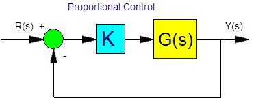
Consider a closed-loop system as shown:

The form of G(s) indicates the process is Type 1 (one integrator present). This means there will be no steady-state error in the step response of the closed-loop system, and the DC gain of the closed-loop will be equal to 1. The closed-loop transfer function is that of the standard 2nd order system with the DC gain equal to 1:
| [latex]G_{cl}(s)=\frac{\omega _{n}^{2}}{s^{2}+2\zeta \omega _{n}+\omega_{n}^{2}}[/latex] |
Equation 12‑1 |
In the frequency domain:
| [latex]G(j\omega)=\frac{\omega _{n}^{2}}{(j\omega)^{2}+2\zeta \omega _{n}(j\omega)+\omega_{n}^{2}}[/latex] |
Equation 12‑12 |
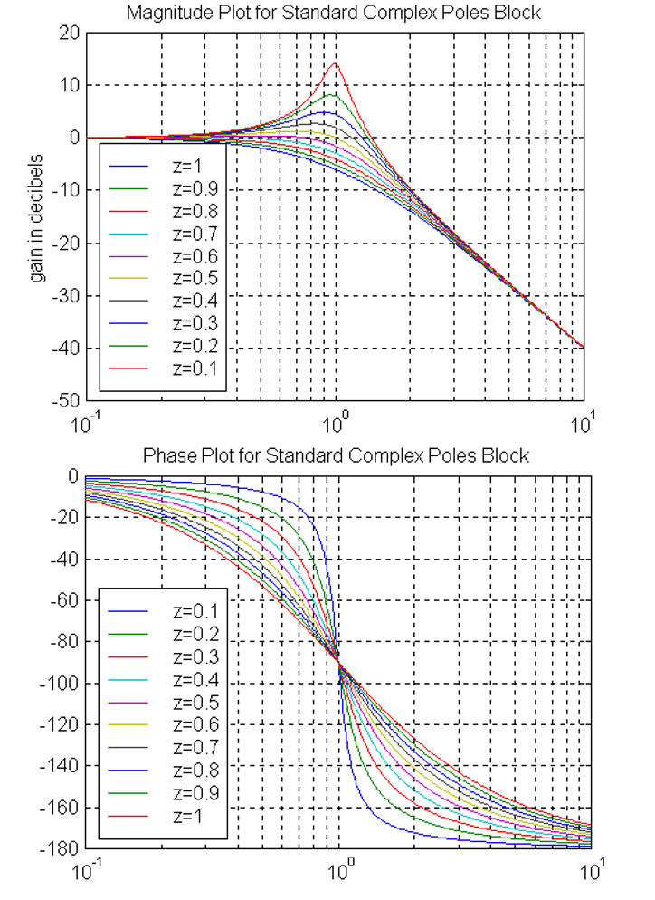
Values of the damping ratio [latex]\zeta[/latex] will affect the shape of the magnitude and phase plots, as shown in Figure 12‑2 for several values of damping ratio between 0 and 1, and for [latex]\omega _{n}=1[/latex]. Small values of the damping ratio [latex]\zeta[/latex] correspond to large resonant peaks on the magnitude plot. Note that linear approximations cannot be used in this case.
For [latex]s=j\omega _{n}[/latex]
|
[latex]G(j\omega _{n})=\frac{\omega _{n}^{2}}{-\omega_{n}^{2}+2\zeta \omega _{n}j\omega _{n}+\omega_{n}^{2}}=[/latex] [latex]\frac{\omega _{n}^{2}}{j2\zeta \omega _{n}^{2}}=\frac{1}{j2\zeta}=\frac{1}{2\zeta}=\angle -90^{0}[/latex] |
Equation 12‑3 |
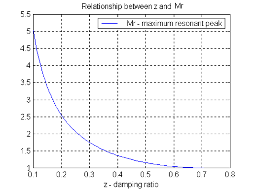
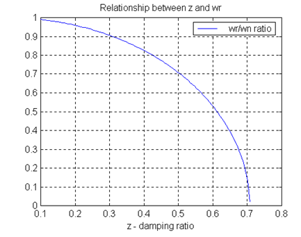
The magnitude is high at frequency [latex]\omega _{n}[/latex], but not at its peak. The maximum magnitude of the resonant peak, [latex]M _{r}[/latex], occurs at the frequency of resonance, [latex]\omega _{r}[/latex]. Relationships between these two parameters and the system parameters [latex]\zeta[/latex], [latex]\omega _{n}[/latex] are as follows:
|
[latex]\omega _{r}=\omega _{n}\sqrt{1-2\zeta ^{2}}[/latex] [latex]M _{r}=\frac{1}{2\zeta \sqrt{1-\zeta ^{2}}}[/latex] |
Equation 12‑4 |
Equation 12‑4 can be derived as follows:
| [latex]M (\omega)=\left | G(j\omega) \right |=\frac{\omega_{n}^{2}}{\sqrt{(\omega_{n}^{2}-\omega^2) ^{2}+(2\zeta\omega_{n}\omega) ^{2}}}[/latex] |
Equation 12‑5 |
To find the maximum of the magnitude function, its derivative is set to zero:
| [latex]\frac{dM(\omega)}{d\omega}=0[/latex] |
Equation 12‑16 |
| [latex]\frac{dM(\omega)}{d\omega}=\omega_{n}^2\left ( \frac{-1}{\left ( \sqrt{(\omega_{n}^{2}-\omega^2) ^{2}+(2\zeta\omega_{n}\omega) ^{2}} \right )^2}. \frac{-1}{2\sqrt{(\omega_{n}^{2}-\omega^2) ^{2}+(2\zeta\omega_{n}\omega) ^{2}}}.\left ( 2(\omega_{n}^{2}-\omega^2)(-2\omega)+8\zeta^2\omega_{n}^2\omega) \right ) \right )[/latex]
[latex]\frac{dM(\omega)}{d\omega}=0 \mapsto (\omega_{n}^{2}-\omega^2) (-\omega )+2\zeta^2\omega_{n}^2\omega=0 \mapsto \omega(-\omega_{n}^2+\omega^2+2\zeta^2\omega_{n}^2)=0[/latex] |
Equation 12-17 |
| [latex]\omega_{r} = \omega_{n}\sqrt{1-2\zeta^2}[/latex] |
Equation 12-18 |
| [latex]M_{r}=M(\omega=\omega_{r})=\frac{\omega_{n}^{2}}{\sqrt{(\omega_{n}^{2}-\omega_{r}^2) ^{2}+(2\zeta\omega_{n}\omega_r) ^{2}}}=[/latex]
[latex]\frac{\omega_{n}^{2}}{\sqrt{(\omega_{n}^{2}-\omega_{n}^{2}(1-2\zeta^2))^2+4\zeta^2\omega_{n}^4(1-2\zeta^2)}}=[/latex] |
Equation 12-19 |
Note that instead of solving Equation 12‑9, readouts of [latex]\omega_{r}[/latex] and [latex]M_{r}[/latex] can be obtained from the plots in Figure 12‑4 and in Figure 12‑3, representing these equations. Knowing [latex]\omega_{r}[/latex] and [latex]M_{r}[/latex] which can also be read off the closed loop frequency response plot, if it is available, the complete closed loop transfer function in Equation 12‑1 can be found.
12.1.2 Dominant Poles Model in Frequency Domain
Consider now a closed loop system as shown:
Process G(s) is now of the order higher than 2nd, and it doesn’t have to be Type 1. In fact, it will most likely be Type 0, as the majority of industrial systems are. If the open loop transfer function is Type 0 (i.e. has no integrator in it), the closed loop system has the DC gain of less than 1. Assume that the resulting closed loop system transfer function will have two dominant complex poles (such assumption holds true for a vast majority of industrial systems), as shown in Figure 12‑5. The DC gain has to be accurately reflected in the system model. As a result, a second order, complex poles transfer function with the DC gain of 1 is no longer appropriate to model the closed loop system.
It has to be modified by adding a multiplier factor to reflect a non-unit DC gain, as shown in Equation 12‑10. The resulting frequency response for this model can be derived in the same way as before. However, since the system transfer function has a non-unit DC gain, while the formula describing the resonant frequency [latex]\omega_{r}[/latex], does not change, the formula describing the maximum of the resonant peak in Equation 12‑4 has to be modified, as shown in Equation 12‑11.

| [latex]G_{cl}(s)\approx K_{dc}\frac{\omega_n^2}{s^2+2\zeta\omega_ns+\omega_n^2}[/latex] | Equation 12‑10 |
|
[latex]M_r=K_{dc}\frac{1}{2\zeta \sqrt{1-\zeta^2}},(\frac{M_r}{K_{dc}})=\frac{1}{2\zeta \sqrt{1-\zeta^2}}[/latex] |
Equation 12‑11 |
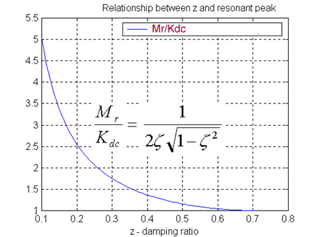
The damping ratio [latex]\zeta[/latex] can be then found either by solving Equation 12‑11, or it can be estimated by a readout from the plot shown in Figure 12‑6. Since magnitude frequency plots are most often shown in dB units, the ratio [latex]\frac{M_r}{K_{dc}}[/latex]can be read off in dB units from the plot as shown in Figure 12‑7 and then converted to V/V units. This allows the proper calculation of the equivalent closed damping ratio [latex]\zeta[/latex] , as shown in Equation 12‑12.
| [latex]\left ( \frac{M_r}{K_{dc}} \right )_{dB}=(M_{r})_{dB}-(K_{dc})_{dB}[/latex] | Equation 12‑12 |
Once the closed loop model described by Equation 12‑10 (system model parameters [latex]K_{dc},\zeta,\omega_{n}[/latex]) is estimated, based on closed loop frequency response and assuming the presence of the dominant complex poles, the important closed loop step response specifications can also be estimated ([latex]PO,T_{rise},T_{settle}[/latex]).

Note that while the closed loop frequency response may not always be directly available from measurements, it can be computed based on the open loop frequency response, which usually is available. The calculations can be easily performed using MATLAB, by converting the measured magnitude-phase data into a complex open loop frequency function [latex]G(j\omega)[/latex], and then by computing the closed loop frequency function and plotting it:
| [latex]G_{cl}(j\omega)=\frac{G(j\omega)}{1+G(j\omega)}[/latex] | Equation 12‑13 |
