
Chapter 14
14.7 Solved Examples of Nyquist Stability Criterion
14.7.1 Example
A unity feedback control system is to work under Proportional Control. The process transfer function is described as follows:
[latex]G(s)= \frac{1}{s^3+2s^2+3s+4}[/latex]
Apply the Nyquist criterion to determine the system closed loop stability. Step 1: Determine the number of unstable open loop poles:
[latex]Q(s)=s^3+2s^2+3s+4=0[/latex]

There are no unstable poles, [latex]P = 0[/latex].
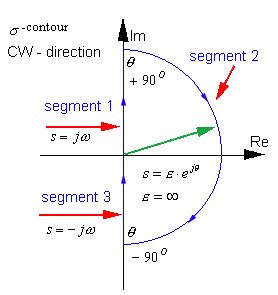
Step 2: Choose the appropriate contour in the s-plane. The [latex]\sigma[/latex]-contour can be divided into several segments:

Segment 1 corresponds to the positive Imaginary axis, i.e.[latex]s=j \omega[/latex] . It maps into [latex]G(s)H(s)[/latex]-plane as a polar plot [latex]G(j \omega )H(j \omega )[/latex]. The polar plot [latex]G(j \omega )H(j \omega )[/latex] can be obtained analytically (tedious), plotted based on Bode plot information (magnitude and phase – just remember that magnitude has to be expressed in Volt/Volt unit, not in dB), or computed using MATLAB.
Segment 3 corresponds to the negative Imaginary axis, i.e. [latex]s=-j \omega[/latex] and its map,[latex]G(-j \omega )H( -j \omega )[/latex] , is a mirror image of the polar plot [latex]G(j \omega )H(j \omega )[/latex] . Segment 2 corresponds to:
[latex]S=\epsilon \cdot e^{j \theta}[/latex]
[latex]\epsilon= \infty[/latex]
Where [latex]\theta[/latex] changes from [latex]+90^ \circ[/latex] to [latex]-90^ \circ[/latex] . Segment 2 typically maps into the origin of the [latex]G(s)H(s)[/latex] map – (0,j0) point, since most systems have more poles than zeros:
Step 3: Map the s-plane contour into the [latex]G(s)H(s)[/latex] plane.
Segment 1 maps into a polar plot, as obtained in the previous example. Segment 2 maps into the origin, and Segment 3 maps into a mirror image of the polar plot, as shown.

The size of the contour will vary depending on the gain [latex]K[/latex]. In Error! Reference source not found., contours are shown for three different values of [latex]K[/latex], [latex]K = 1[/latex], [latex]K = 2[/latex], and [latex]K = 5[/latex].

It is easier however to retain the same contour [latex]G(s)H(s)[/latex] and scale the Real and Imaginary axis in the [latex]G(s)H(s)[/latex]-plane.

Step 4: Apply the Nyquist Criterion. When the plot is scaled for Proportional Gain [latex]K[/latex], four different areas can be analyzed:
| [latex]- \infty < - \frac{1}{K} < -0.5[/latex] | [latex]0< K <+2[/latex] | Z = N+P = 0 + 0 = 0 | stable |
| [latex]- 0.5< - \frac{1}{K} <0[/latex] | [latex]+2| Z = N+P = 2+ 0 = 2 |
unstable |
|
| [latex]0< - \frac{1}{K}<+0.25[/latex] | [latex]- \infty| Z = N+P = 1+ 0 = 1 |
unstable |
|
| [latex]0.25<- \frac{1}{K}<+ \infty[/latex] | [latex]-4| Z = N+P = 0 + 0 = 0 |
stable |
|
Based on the Nyquist Stability Criterion, two ranges of [latex]K[/latex] values for stable system operation have been found (only one practical, for [latex]K > 0[/latex]):
[latex]2-K>0[/latex] [latex]K<2[/latex]  [latex]-4
[latex]K+4>0[/latex] [latex]K>-4[/latex]
14.7.2 Example
Consider the same system as before, where a unity feedback control system is to work under Proportional Control, with the process transfer function described as follows:
[latex]G(s)= \frac{10}{s^3+4s^2+6s+8}[/latex]
Apply the Nyquist criterion to determine the system closed loop stability.
Solution
Step 1: Determine the number of unstable open loop poles, [latex]P[/latex]:
[latex]Q(s)=s^3+4s^2+6s+8=0[/latex]

Step 2: Choose the appropriate contour in the s-plane.
Step 3: Map the contour into the [latex]G(s)H(s)[/latex] plane. Use the information provided in the open loop frequency plots. Segment 1 maps into the system polar plot, as obtained in Example 14.3.3. Segment 2 maps into the origin, and Segment 3 maps into a mirror image of the polar plot.

Step 4: Apply the Nyquist Criterion. When the plot is scaled for Proportional Gain [latex]K[/latex], four different areas can be analyzed:
| [latex]- \infty < - \frac{1}{K} < -0.625[/latex] | [latex]0< K <+1.6[/latex] | Z = N+P = 0 + 0 = 0 | stable |
| [latex]- 0.625< - \frac{1}{K} <0[/latex] | [latex]+1.6| Z = N+P = 2+ 0 = 2 |
unstable |
|
| [latex]0< - \frac{1}{K}<+1.25[/latex] | [latex]- \infty| Z = N+P = 1 + 0 = 1 |
unstable |
|
| [latex]+1.25<- \frac{1}{K}<+ \infty[/latex] | [latex]-0.8| Z = N+P = 0 + 0 = 0 |
stable |
|
Based on the Nyquist Stability Criterion, the system is stable for:
[latex]-0.8
Consider the system from Example 14.3.4, of a unity feedback control system under Proportional Control, with the process transfer function described as follows:
[latex]G(s)= \frac{5}{s(s+1)(s+5)}[/latex]
Apply Nyquist stability criterion to this system.
Solution:
The polar plot of this system was established in Example 14.3.4. Note that because it is a Type I system, its open loop pole sits at the origin of the s-plane. Choose the [latex]\sigma[/latex]-contour encircling the whole of the unstable region, RHP, avoiding going through the origin of the s-plane – one of the system singularities (integrator) is there. We can encircle the origin with a radius of zero on either left or right side. The contour below encircles the origin on the right, as shown. There are no unstable open loop poles of [latex]G(s)[/latex] in this contour, P = 0. Note that if we chose to encircle the origin of the s-plane to the left, we would end up with 1 unstable open loop pole inside the contour. There are four segments of the [latex]\sigma[/latex]-contour to be mapped.
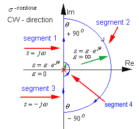
Segment 1 corresponds to the positive Imaginary axis, i.e. [latex]s=j \omega[/latex] . It maps into [latex]G(s)H(s)[/latex]-plane as a polar plot [latex]G(j \omega )[/latex] .
Segment 3 corresponds to the negative Imaginary axis, i.e. [latex]s=-j \omega[/latex] and its map, [latex]G(-j \omega )H(-j \omega )[/latex], is a mirror image of the polar plot [latex]G(j \omega )H(j \omega )[/latex]. Segment 2 corresponds to:
[latex]S= \epsilon \cdot e^{j \theta }[/latex]
[latex]\epsilon = \infty[/latex]
Where [latex]\theta[/latex] changes from [latex]+90^ \circ[/latex] to [latex]-90^ \circ[/latex] . Segment 2 maps into the origin of the [latex]G(s)H(s)[/latex] map – (0,j0) point, since the system has three poles.
Segment 4 corresponds to the minuscule encirclement to the right of the origin: [latex]S= \epsilon \cdot e^{j \theta}[/latex] , [latex]\epsilon=0[/latex], where [latex]\theta[/latex] changes from [latex]-90^ \circ[/latex] to [latex]+90^ \circ[/latex] . Since magnitude of [latex]s[/latex] approaches zero, the shape of the resulting [latex]G(s)[/latex] contour will have an infinite radius. We need to figure out which way it circles in the [latex]G(s)[/latex] plane:
[latex]\lim\limits_{s \rightarrow 0} G(s)= \lim\limits_{s \rightarrow 0} \frac{5}{s(s+1)(s+5)}= \lim\limits_{s \rightarrow 0} \frac{5}{s(1)(5)} = \lim\limits_{s \rightarrow 0} \frac{1}{s}[/latex]
[latex]\mid \lim\limits_{s \rightarrow 0} \frac{1}{s} \mid = \infty[/latex]
[latex]\angle ( \lim\limits_{s \rightarrow 0 } G(s))= \angle ( \frac{1}{s} ) = - \angle (s) = - \theta[/latex]
|
[latex]\angle (s) = \theta[/latex] |
[latex]\angle ( \lim\limits_{s \rightarrow 0}G(s))= \angle ( \frac{1}{s} )[/latex] |
|
[latex]\theta = -90^ \circ[/latex] |
[latex]\angle ( \frac{1}{s} ) = +90^ \circ[/latex] |
|
[latex]\theta = 0^ \circ[/latex] |
[latex]\angle ( \frac{1}{s} ) = 0^ \circ[/latex] |
|
[latex]\theta = +90^ \circ[/latex] |
[latex]\angle ( \frac{1}{s} ) = -90^ \circ[/latex] |
This table tells us that as we follow Segment 4 of the [latex]\sigma[/latex]-contour, it maps into a [latex]G(s)[/latex]-plane contour, which is a clock wise (CW) half-circle with an infinite radius. The complete Nyquist contour for this system is shown next.

There are three areas for analysis of the relative position of the Nyquist contour and the (-1/K,j0) point:
| [latex]- \infty < - \frac{1}{K} < -0.1667[/latex] | [latex]0< K <+6[/latex] | Z = N+P = 0 + 0 = 0 | stable |
| [latex]- 0.1667< - \frac{1}{K} <0[/latex] | [latex]6| Z = N+P = 2+ 0 = 2 |
unstable |
|
| [latex]+0< - \frac{1}{K}<+ \infty[/latex] | [latex]- \infty | Z = N+P = 1+ 0 = 1 |
unstable |
|
Based on the Nyquist Stability Criterion, the system is stable for [latex]0
Consider the system with the unit feedback closed loop system under Proportional Gain as before, where the open loop transfer function [latex]G(s)[/latex] is known to be unstable and its transfer function [latex]G(s)[/latex] is known as
[latex]G(s)= \frac{s+2}{s(s-2)}[/latex]
Apply the Nyquist Criterion of Stability to this system.
Solution
Choose the [latex]\sigma[/latex] -contour encircling the whole of the unstable region, RHP, avoiding going through the origin of the s-plane – one of the system singularities (integrator) is there. We can encircle the origin with a radius of zero on either the left or right side. The contour below encircles the origin on the right.
There is one unstable open loop pole of [latex]G(s)[/latex] in this contour (pole at +2,j0), i.e. P = 1. Note that if we chose to use the contour encircling the origin to the left, two unstable open loop poles would be included inside the [latex]\sigma[/latex] -contour. There are four segments of the [latex]\sigma[/latex]-contour to be mapped. Segment 1 corresponds to the positive Imaginary axis, i.e. [latex]s=j \omega[/latex]. It maps into [latex]G(s)H(s)[/latex]-plane as a polar plot [latex]G(j \omega )[/latex]. The polar plot [latex]G(j \omega )[/latex] can be obtained analytically (tedious), plotted based on Bode plot information (magnitude and phase – just remember that magnitude has to be expressed in Volt/Volt unit, not in dB), or computed using MATLAB. Let’s try the analytical approach for a change.

In frequency domain [latex]G(s)[/latex] can be expressed as
[latex]G(j \omega )= \frac{j \omega +2}{(j \omega)(j \omega -2)}[/latex]
[latex]G(j \omega )= \frac{(j \omega +2)(-2-j \omega )}{j \omega (j \omega -2)(-2-j \omega )}=[/latex] [latex]\frac{(j \omega +2)(-2-j \omega )}{ \omega (j \omega -2)(-2-j \omega )} (-j)=[/latex]
[latex]=- \frac{4}{4+ \omega^2}-j \frac{ \omega^2 -4}{ \omega ( \omega^2 +4)}[/latex]
[latex]Re \{G(j \omega ) \} = - \frac{4}{4+ \omega^2}[/latex]
[latex]Im \{(j \omega ) \} = - \frac{ \omega^2-4}{ \omega ( \omega^2 +4)}[/latex]
Based on the above equations, the polar plot starts at [latex](-1,+j \infty )[/latex] for frequency [latex]\omega =0[/latex], crosses over the Real axis at [latex]\omega =2[/latex] rad/s at the coordinate (-0.5,j0), and ends in the origin (0,j0) at [latex]\omega = + \infty[/latex]. We can arrive at the same conclusion simply by checking the open loop frequency plots, shown again below.
To sketch the polar plot using Bode plot information, write appropriate values of important frequencies and corresponding magnitudes and phases in a table like the one below:
| frequency | Magnitude in dB | Magnitude V/V | Phase in degrees |
| [latex]\omega =0[/latex] | [latex]+ \infty[/latex] | [latex]+ \infty[/latex] | [latex]-270^ \circ[/latex] |
| [latex]\omega =2[/latex] rad/s | [latex]-6[/latex] dB | [latex]0.5[/latex] Volt/Volt | [latex]-180^ \circ[/latex] |
| [latex]\omega = + \infty[/latex] | [latex]- \infty[/latex] | [latex]0[/latex] | [latex]-90^ \circ[/latex] |

The polar plot corresponding to Segment 1 of the s-plane contour can then be sketched. Segment 2 corresponds to
[latex]S= \epsilon \cdot e^{j \theta }[/latex]
[latex]\epsilon = \infty[/latex]
where [latex]\theta[/latex] changes from [latex]+90^ \circ[/latex] to [latex]-90^ \circ[/latex]. Segment 2 maps into the origin of the [latex]G(s)H(s)[/latex] map – (0,j0) point, since the system has two poles and only one zero. Segment 3 corresponds to the negative Imaginary axis, i.e. [latex]s=-j \omega[/latex] and its map, [latex]G(-j \omega )H(-j \omega )[/latex], is a mirror image of the polar plot [latex]G(j \omega )H(j \omega )[/latex]. Segment 4 corresponds to the minuscule encirclement to the right of the origin:
[latex]s= \epsilon \cdot e^{j \theta }[/latex]
[latex]\epsilon =0[/latex]
where [latex]\theta[/latex]; changes from [latex]-90^ \circ[/latex] to [latex]+90^\circ[/latex]. Since the magnitude of s approaches zero, the shape of the resulting [latex]G(s)[/latex] contour will have an infinite radius.

We need to figure out which way it circles in the [latex]G(s)[/latex] plane:
[latex]\lim\limits_{s \rightarrow 0} G(s) = \lim\limits_{s \rightarrow 0} \frac{s+2}{s(s-2)} = \lim\limits_{s \rightarrow 0} \frac{2}{s(-2)} = - \lim\limits_{s \rightarrow 0} \frac{1}{s}[/latex]
[latex]\mid \lim\limits_{s \rightarrow 0} \frac{1}{s} \mid = \infty[/latex]
[latex]\angle ( \lim\limits_{s \rightarrow 0} G(s)) = \angle ( \frac{1}{s} ) +180^ \circ = - \angle (s) +180^ \circ = - \theta +180^ \circ[/latex]
| [latex]\angle (s)= \theta[/latex] | [latex]( \lim\limits_{s \rightarrow 0 } G(s))= \angle ( \frac{1}{s})+180^ \circ[/latex] |
| [latex]\theta = -90^ \circ[/latex] | [latex]\angle ( \frac{1}{s} )= +90^ \circ + 180^ \circ=+270^ \circ[/latex] |
| [latex]\theta = 0^ \circ[/latex] | [latex]\angle ( \frac{1}{s} )= 0^ \circ + 180^ \circ=+180^ \circ[/latex] |
| [latex]\theta = +90^ \circ[/latex] | [latex]\angle ( \frac{1}{s}) = -90^ \circ+180^ \circ = +90^ \circ[/latex] |
This table tells us that as we follow Segment 4 of the [latex]\sigma[/latex] -contour, it maps into a [latex]G(s)[/latex]-plane contour, which is a counter-clock wise (CCW) half-circle with an infinite radius. The complete Nyquist contour for this system is shown next. There are three areas for analysis of the relative position of the Nyquist contour and the (-1/K,j0) point:
| [latex]- \infty < - \frac{1}{K} < -0.5[/latex] | [latex]0< K <2[/latex] | Z = N+P = 1 + 1 = 2 | unstable |
| [latex]- 0.5< - \frac{1}{K} <0[/latex] | [latex]2| Z = N+P = -1+ 1 = 0 |
stable |
|
| [latex]+0< - \frac{1}{K}<+ \infty[/latex] | [latex]- \infty | Z = N+P = 0+ 1 = 1 |
unstable |
|
Based on the Nyquist criterion, the system is stable for [latex]2
