
Chapter 13
13.4 Lag Controller
A transfer function of the Lag Controller is as follows, where [latex]a_0 = K_c[/latex] corresponds to the DC gain of the controller, and [latex]\alpha < 1[/latex] – the pole is closer to Im axis than the zero:
| [latex]G_c(s)=\frac{a_1 s + a_0}{b_1 s + 1}=K_c\frac{s\alpha\tau +1}{s\tau+1}[/latex] | Equation 13-16 |
Zero is at [latex]s_1 = -\frac{a_0}{a_1}=-\frac{1}{\alpha\tau}[/latex], pole is at [latex]s_2 = -\frac{1}{b_1}=-\frac{1}{\tau}[/latex] as shown in Figure 13‑18.

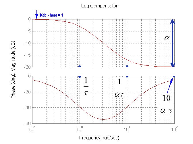
In the frequency domain, the two corner frequencies are: [latex]\omega_1 = \frac{1}{\alpha\tau}[/latex], [latex]\omega_2=\frac{1}{\tau}[/latex]
The magnitude is described as:
| [latex]G_c(s)=K_c \cdot \frac{s\alpha\tau +1}{s\tau+1}[/latex]
[latex]M(\omega)=K_c\cdot\frac{\sqrt{{(\omega\alpha\tau)}^2 + 1}}{\sqrt{{(\omega\tau)}^2 + 1}}[/latex] |
Equation 13‑17 |
The phase is described as:
| [latex]\phi(\omega)=\tan^{-1}\omega\alpha\tau - \tan^{-1}\omega\tau[/latex] | Equation 13‑18 |
The approximate end of the phase lag occurs at the frequency:
| [latex]\omega_1 = \frac{10}{\alpha\tau}[/latex] | Equation 13‑19 |
This frequency then will be positioned over the chosen crossover frequency [latex]\omega_{cp}[/latex]. The gain drop added by the lag component (with respect to its DC gain level) is equal to:
| [latex]M(\omega)=K_c\cdot\frac{\sqrt{{(\omega\alpha\tau)}^2 + 1}}{\sqrt{{(\omega\tau)}^2 + 1}}\;\omega \rightarrow \infty[/latex]
[latex]M(\omega)\approx K_c\cdot\frac{\sqrt{{(\omega\alpha\tau)}^2}}{\sqrt{{(\omega\tau)}^2}} = K_c\cdot\alpha[/latex] |
Equation 13‑20 |
Frequency response plots of the Lag Controller (without its DC gain, [latex]K_{dc}[/latex]) are shown in Figure 13‑19.
How to use the Lag Controller:
- Use the Lag Controller gain, [latex]K_c[/latex] to correct deficiencies in the steady state tracking.
- Use the Lag Controller parameter to adjust the dynamic gain for the correct crossover [latex] \omega_{cp}[/latex] and Phase Margin [latex]\Phi_m[/latex].
- Adjust as required.
13.4.1 Simplified Lag Controller Design
For the simplified design, this form of the Lag Compensator is more useful:
| [latex]G_c(s)=K_c\cdot\frac{\tau\alpha s +1}{\tau s +1}[/latex] |
Equation 13‑21 |
Zero is at [latex]s_1 = -\frac{1}{\alpha\tau}[/latex], pole is at [latex]s_2 = -\frac{1}{\tau}[/latex] as shown in Figure 13‑18. The design will involve making a decision on what the compensated system phase margin [latex]\Phi_m[/latex] should be and what the steady state tracking accuracy should be. The lag network contributes a negative angle, so it has to be positioned over the frequency response of a process to be compensated in such a way that its angle contribution to the overall compensated angle is zero. Otherwise, if the compensated phase angle at the crossover frequency [latex]\omega_{cp}[/latex] is reduced, the system will have a smaller phase margin, and thus the equivalent damping ratio of the closed loop system will be worse.
The steps involved in the compensation process are as follows. First, the open loop frequency response is adjusted by the required DC gain (determined based on the steady state error requirements).
Next, from the plot of the open loop frequency response, [latex]G(j\omega)[/latex], the frequency of crossover is chosen such that an appropriate phase margin (plus an extra 5 degrees) can be provided by the process phase itself:
| [latex]\angle G(j\omega) = -180^{\circ}+\Phi_m+5^{\circ}[/latex] | Equation 13-22 |
Once this frequency is determined, the Lag Controller parameter is calculated based on the gain drop required. Finally, since the end of the lag phase of the Lag Controller is at the crossover frequency, we have:
| [latex]\omega_{cp} = \omega_1 = \frac{10}{\alpha\tau}[/latex] | Equation 13-23 |
13.4.2 Analytical Lag Controller Design
An alternative approach to the Lag Controller is to use the same design equations as for the Lead Controller, with the new crossover frequency [latex]\omega_{cp}[/latex] chosen to be smaller than the uncompensated one. For the analytical design, this form of the Lag Controller is used:
| [latex]G_c(s)=\frac{a_1 s + a_0}{b_1 s + 1}[/latex] | Equation 13-24 |
Note that [latex]a_0=K_c[/latex] corresponds to the DC gain of the controller. Zero is at [latex]s_1 = - \frac{a_0}{a_1}[/latex], pole is at [latex]s_2 = - \frac{1}{b_1}[/latex].
| [latex]\theta = -180^{\circ}+\Phi_m-\angle G(j\omega_{cp})[/latex] | Equation 13-25 |
Calculate the Lag Controller coefficients:
| [latex]a_1 = \frac{1-a_0\cdot \left| G(j\omega_{cp}) \right | \cdot \cos{\theta}}{\omega_{cp}\cdot \left| G(j\omega_{cp}) \right | \cdot \sin{\theta}}[/latex]
[latex]b_1 = \frac{\cos{\theta})-a_0\cdot \left| G(j\omega_{cp}) \right |}{\omega_{cp}\cdot \sin{\theta}}[/latex] |
Equation 13-26 |
Observation I:
The same as in the case of Lead Controller: if either coefficient < 0, iterations are necessary.
Observation II:
Note that if [latex]\omega_{cp}[/latex] for the compensated system is chosen to be larger than that of the uncompensated system, we will end up with a Lead Controller (where the zero is closer to Im axis than the pole).
