
Chapter 7
7.1 Second Order Underdamped Systems
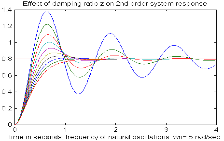
Consider a second order system described by the transfer function in Equation 7‑1, where [latex]\zeta[/latex] is called the system damping ratio, and [latex]\omega_{n}[/latex] is called the frequency of natural oscillations. We will later show that the system oscillation depends on the value of the damping ratio [latex]\zeta[/latex]. The underdamped second order system step response is shown in Figure 7‑1 where different colours correspond to different damping ratios – the smaller the damping, the larger the oscillation.
| [latex]G(s) = K_{dc}\frac{\omega^{2}_{n}}{s^{2} + 2\zeta\omega s + \omega_{n}^{2}}[/latex] | Equation 7-1 |
Recall that the solution for quadratic roots is as follows:
[latex]ax^{2} + bx + c = 0[/latex]
[latex]\Delta = b^{2} - 4ac[/latex]
Depending on the value of [latex]\Delta[/latex], we will have three distinct cases:
- if [latex]\Delta > 0[/latex], there are two real, distinct roots. Note that this would be a case with the previously discussed, second order system where we identified two Time Constants. Its response is referred to as an overdamped response, and the system is called an overdamped 2nd order system, where the two poles are:
[latex]x_{1} = \frac{-b-\sqrt{\Delta}}{2a}, x_{2} = \frac{+b+\sqrt{\Delta}}{2a}[/latex]
- if [latex]\Delta = 0[/latex], there are two identical roots, or we can say one double root. The response is referred to as a critically damped response, and the system is called a critically damped system, with a double pole:
[latex]x_{1} = x_{2} = \frac{-b}{2a}[/latex]
- if [latex]\Delta < 0[/latex], there are two complex, conjugate roots, and the response is a sinusoid with an exponential envelope. This oscillatory response is called an underdamped response, and the system is called a second order underdamped system where the two poles are:
[latex]x_{1} = \frac{-b-j\sqrt{-\Delta}}{2a}, x_{2} = \frac{+b+j\sqrt{-\Delta}}{2a}[/latex]
Applying the quadratic roots solution to the denominator of G(s), we have:
| [latex]s^{2} + 2\zeta\omega_{n}s + \omega_{n}^{2} = 0[/latex] | |
| [latex]\Delta = (2\zeta\omega_{n})^{2} - 4 \cdot 1 \cdot \omega_{n}^{2} = 4\zeta^{2}\omega_{n}^{2} - 4\omega_{n}^{2} = 4\omega_{n}^{2}(\zeta^{2} - 1)[/latex] | |
| [latex]\sqrt{\Delta} = \sqrt{4\omega^{2}_{n}(\zeta^{2}-1)} = 2\omega_{n}\sqrt{\zeta^{2}-1}[/latex] | Equation 7-2 |
Again, depending on the value of [latex]\zeta[/latex], we will have these three distinct cases.
- If [latex]\zeta > 1[/latex] then [latex]\Delta > 0[/latex] and the roots are real (i.e. the system is overdamped with two real poles, and there are two exponentially damped transients);
- If [latex]\zeta = 1[/latex] then [latex]\Delta > 0[/latex] and the roots are real and identical (i.e. the system is critically damped with two equal real poles, and there are two transients – one is an exponential, the other is time multiplied by an exponential)
- If [latex]\zeta < 1[/latex] then [latex]\Delta < 0[/latex] and the roots are complex conjugates (i.e. the system is underdamped with two complex poles, and the transient is an exponentially damped sinusoid);
| [latex]s_{1} = -\zeta\omega_{n} - j\omega_{n}\sqrt{1-\zeta^{2}} = \-\zeta\omega_{n} - j\omega_{d}[/latex] | |
| [latex]s_{1} = -\zeta\omega_{n} + j\omega_{n}\sqrt{1-\zeta^{2}} = \-\zeta\omega_{n} + j\omega_{d}[/latex] | Equation 7-3 |
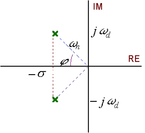
The overdamped case was discussed in Chapter 6.2. It is of no particular interest in Control Systems design because the system response time is slow – the system speed is measured by the Rise time and the Settling Time. The critically damped case cannot be visually identified from the overdamped case and is of interest only as the borderline behaviour between the two distinct cases: overdamped and underdamped responses. From the point of view of Control Systems Design, only the latter is of interest, as an underdamped system has fast response times. The downside of course is that the faster it is, the less damping, and therefore it is more oscillatory, but in the design part we will learn to “fix” that. Transfer function G(s) in Equation 7‑1 has two complex poles and no zeros. The pole locations in the complex plane are shown in Figure 7‑2. In it, [latex]\sigma = \zeta\omega_{n}[/latex] is called a decay rate. Its inverse, [latex]\tau = \frac{1}{\sigma} = \frac{1}{\zeta\omega_{n}}[/latex] is called the time constant of the system.
The pole locations in the complex plane are shown in Figure 7‑2. In it, [latex]\sigma = \zeta \omega_{n}[/latex] is called a decay rate. Its inverse, [latex]\tau = \frac{1}{\sigma} = \frac{1}{\zeta \omega_{n}}[/latex] is called the time constant of the system.
[latex]\sigma = \zeta \omega_{n}[/latex]
[latex]cos\phi = \frac{\zeta \omega_{n}}{\omega_{n}} = \zeta[/latex]
[latex]sin\phi = \frac{\omega_{n} \sqrt{1-\zeta^{2}}}{\omega_{n}} = \sqrt{1 - \zeta^{2}}[/latex]
Note that the damping ratio [latex]\zeta[/latex] can be calculated from the trigonometrical relationship shown in Figure 7‑2.
| [latex]cos\phi = \frac{\zeta\omega_{n}}{\omega_{n}} = \zeta[/latex] | |
| [latex]\ phi = cos^{-1}\zeta[/latex] | Equation 7-4 |
The unit step response of G(s) can be derived using standard Table of Laplace Transforms:
| [latex]Y_{step}(s) = \frac{1}{s}\cdot K_{dc} \cdot \frac{\omega^{2}_{n}}{s^{2} + 2\zeta\omega_{n}s + \omega^{2}_{n}}[/latex] | |
| [latex]y_{step}(s) = L^{-1}\Bigg\{ Y_{step}(s)\Bigg\}[/latex] | |
| [latex]y_{step}(t) = K_{dc}\cdot \Bigg( 1 - \frac{e^{-\zeta\omega_{n}t}}{\sqrt{1-\zeta^{2}}}sin\bigg(\omega_{n}\sqrt{1-\zeta^{2}}t + cos^{-1}\zeta\bigg)\Bigg)\cdot 1(t)[/latex] | Equation 7-5 |
If the unit step input is used, the process DC gain and time constant can be evaluated directly from the graph, as was illustrated in previous chapters. We will now demonstrate that the damping ratio and the frequency of natural oscillations can be evaluated from the response plot as well.
