
Chapter 9
9.2 Proportional Control
Figure 9‑9 shows a basic closed loop configuration with a proportional Controller.

We looked at the operation of the closed loop system under Proportional Control before, so this is just a recap. Consider an example where the process transfer function is as follows:
| [latex]G(s)=\frac{2}{s^2+5s+2}\cdot\frac{5}{s^2+10s+2}[/latex] | Equation 9-3 |
The closed loop system transfer function is then calculated as:
| [latex]G_{cl(P)}(s)=\frac{K_p G_1(s) G_2(s)}{1+K_p G_1(s) G_2(s)}=\frac{10K_p}{s^4+15s^3+54s^2+30s+(4+10K_p)}[/latex] | Equation 9-4 |
The critical gain can be calculated from the Routh-Hurwitz Criterion as [latex]K_{crit}=10[/latex] and the resulting frequency of marginal oscillations is calculated as [latex]\omega_{osc} = 1.41[/latex] rad/sec. Figure 9‑10 shows the effect of Proportional Control on the closed loop step response of this system – when the controller gain is increased, we see a trade-off between better steady state tracking and worsening transient response and corresponding reduction in the system relative stability (Gain Margin is reduced as gain increases). Working with high gain values is not satisfactory as well because of real-life effects such as possible controller output saturation which makes the control less effective as the system is no longer linear.
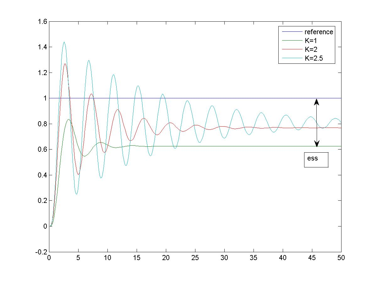
Figure 9‑11 shows the same system response in presence of a disturbance. As Equation 9‑5 shows, the closed loop response of an LTI system is a superposition of the responses to reference and to disturbance signals. In the steady state, ideally, we would want the reference-to-output transfer function to be equal to 1, in order to perfectly duplicate the reference. When the disturbance occurs, we cannot do anything about it as by definition, it is an unknown signal. Therefore, to reduce its effect on the system output, ideally, we would want the disturbance-to-output transfer function to be zero.
| [latex]G_{cl}(s)=\frac{Y(s)}{R(s)}\rvert_{D(s)=0} = \frac{K_p G(s)}{1+K_p G(s)}[/latex] | |
| [latex]G_{dist}(s)=\frac{Y(s)}{D(s)}\rvert_{R(s)=0} = \frac{G(s)}{1+K_p G(s)}[/latex] | |
| [latex]Y(s)=G_cl(s)\cdot R(s)+G_{dist}(s)\cdot D(s)[/latex] | |
| [latex]Y(s)= \frac{K_p G(s)}{1+K_p G(s)}\cdot R(s)+\frac{G(s)}{1+K_p G(s)}\cdot D(s)[/latex] | Equation 9-5 |
As seen in As Equation 9‑5, when the Proportional Gain increases, the steady state value of the closed loop gain (DC gain for the reference-to-output transfer function) will increase, thus improving the steady state tracking of the reference. Similarly, the steady state value of the disturbance-to-output transfer function decreases. Theoretically, when [latex]K_p \rightarrow \infty[/latex], [latex]K_{DC}=G_{cl}(0)\rightarrow 1[/latex] and when [latex]G_{dist}(0)\rightarrow 0[/latex]. Of course, realistically, before that happens, the system will either become unstable or will saturate. Nevertheless, the gain increase does result in the reduction of the disturbance effect on the steady state system response, however, the trade-off again is more transient oscillations in response to disturbance signal.

9.2.1 Summary of Proportional Control Attributes
Steady State Tracking
- High proportional gain – small steady state error
- Low proportional gain – large steady state error
Dynamic Tracking
- High proportional gain – increased system oscillations – can lead to instability
- High proportional gain – undesirable (strong) control effort – may saturate the controller
- High proportional gain – wear and tear of equipment
- Low proportional gain – sluggish, overdamped response
Disturbance Rejection
- High gain needed to reduce the effect of disturbance on the steady state tracking
- High gain – undesirable: lower stability, possibility of saturation, oscillations
