14.6 Cauchy’s Mapping Theorem

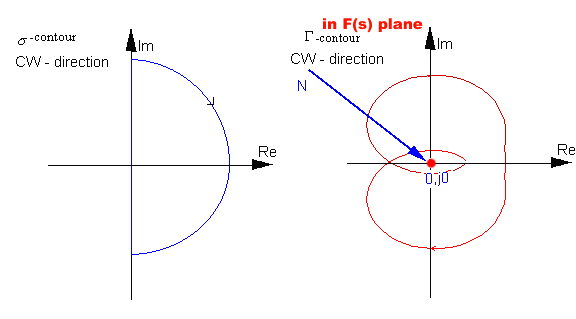
Let’s summarize the above cases. Consider an arbitrarily closed contour [latex]\sigma[/latex] in the s-plane, traversed clockwise (CW), so that it does not go through any singularities of [latex]F(s)[/latex]. Let [latex]Z[/latex] be a number of zeros of [latex]F(s)[/latex] inside the [latex]\sigma[/latex] -contour, and [latex]P[/latex] be a number of poles of [latex]F(s)[/latex] inside the [latex]\sigma[/latex]-contour. Mapping the [latex]\sigma[/latex]-contour into the [latex]F(s)[/latex] plane will result in a closed [latex]\Gamma[/latex]-contour. Let [latex]N[/latex] be a number of clockwise (CW) encirclements of the resulting [latex]\Gamma[/latex]-contour around the origin of the [latex]F(s)[/latex]-plane. The total number of encirclements of the origin of [latex]F(s)[/latex]-plane through the above mapping is equal to:

14.6.1 How Does Cauchy’s Mapping Theorem Apply to a Control System Stability?

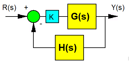
Consider a closed loop system:

The characteristic equation is:

[latex]1+ G(s)H(s)=0[/latex]

[latex]G(s)H(s)= \frac{N_{open}(s)}{D_{open}(s)}[/latex]

[latex]1+ \frac{N_{open}(s)}{D_{open}(s)}=0[/latex]

[latex]\frac{D_{open}(s)+N_{open}(s)}{D_{open}(s)}=0[/latex]

[latex]N_{char}(s)=D_{open}(s)+N_{open}(s)[/latex]

[latex]D_{char}(s)=D_{open}(s)[/latex]

Define a map (function) [latex]F(s)[/latex] such that it is described by a characteristic equation of the closed loop:

Note that the roots of the numerator of the map [latex]F(s)[/latex] are equivalent to closed loop poles and that the roots of the denominator of the map [latex]F(s)[/latex] are equivalent to open loop poles. Now consider taking a [latex]\sigma[/latex]-contour such that it encompasses all of the RHP, as shown:

Typically, the open loop pole locations are known, i.e. P is a known number of unstable open loop poles – we can count how many open loop poles are within this contour. The closed loop pole locations are unknown, i.e. Z is what we want to find out. However, from Cauchy’s Theorem:

[latex]Z=N+P[/latex]

The question then is, how to find N? If we can perform the mapping into [latex]F(s)[/latex]-plane, N  can be simply counted. While the mapping into [latex]F(s)[/latex] (closed loop characteristic equation) is not simple, mapping into [latex]G(s)H(s)[/latex] is very simple – we will use a polar plot to do that. Note that:

[latex]F(s)= 1+ \frac{N_{open}(s)}{D_{open}(s)}=1+ G(s)H(s)[/latex]

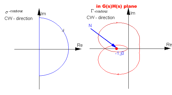
Map [latex]F(s)[/latex] can then be obtained from the map [latex]G(s)H(s)[/latex] by a linear translation by [latex]-1[/latex]. Map [latex]G(s)H(s)[/latex] is easily obtained through frequency response. So, rather than watching the number  N  of CW encirclements of the origin of [latex]F(s)[/latex] plane, we will be watching the number N of CW encirclements of the (-1,j0) point in the [latex]G(s)H(s)[/latex]-plane.

Remember that Z represents the total number of zeros of the [latex]F(s)[/latex] map inside the chosen [latex]\sigma[/latex]-contour in the s-plane, i.e. in the RHP (unstable region). Since the map [latex]F(s)[/latex] was defined for the closed loop characteristic equation, its zeros represent closed loop poles of the control system. Z then represents the total number of unstable closed loop poles of the system.

Since [latex]Z = N + P[/latex], for the system to be stable, Z must be equal to zero, i.e. N + P = 0, or  N = -P.  

We can then define the following stability criterion:

Take a closed [latex]\sigma[/latex] -contour in the s-plane in a CW direction so that it encompasses all of RHP. Obtain the Nyquist contour in the [latex]G(s)H(s)[/latex] plane through mapping (utilize frequency response – polar plots – to do so).

For stability, the Nyquist contour for the closed loop control system with P unstable open loop poles must encircle the (-1,j0) point in [latex]G(s)H(s)[/latex]-plane P times in CCW direction.

Typically, we are not interested in the absolute system stability (i.e. is the system stable or not?), but in the relative system stability (i.e. what is the range of gains [latex]K[/latex] for which this system is stable?):