
Chapter 1
1.5 Transfer Function Representations of Simple Physical Systems
1.5.1 Electrical Systems
Modelling of electrical systems is based on:
- Ohm’s Law
- Kirchhoff’s Current Law (KCL)
- Kirchhoff’s Voltage Law (KVL)
| [latex]V=iR[/latex] | [latex]i = \frac{V}{R}[/latex] | Energy dissipated through resistance as heat. | |
| [latex]V_{L} = L\frac{di}{dt}[/latex] | [latex]i_{L}=\frac{1}{L}\int_{-\infty}^{t} V_{L}dt[/latex] | Energy stored in the magnetic field. No instantaneous change in current. | |
 |
[latex]V_{C}=\frac{1}{C}\int_{-\infty}^{t} i_{C}dt[/latex] | [latex]i_{C} = C\frac{dV}{dt}[/latex] | Energy stored in the electrostatic field. No instantaneous changes in voltage. |
1.5.2 Mechanical Systems
Modelling of mechanical translational systems is based on:
- Newton’s First Law
- Newton’s Second Law
- Free Body Diagrams.
- In Table 1-4 below, we have: [latex]F[/latex]-force, [latex]x[/latex]– translational displacement, [latex]v[/latex]– velocity, [latex]a[/latex]-acceleration
| [latex]F = Bv = B\dot{x}[/latex] | Energy dissipated through viscous damping as heat | |
| [latex]F_{K} = K\int vdt = Kx[/latex] | Energy stored as kinetic-potential | |
| [latex]F = Ma = M\dot{v} =M\ddot{x}[/latex] | Energy stored as kinetic-potential |
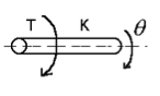
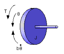
1.5.3 Mechanical Rotational Systems
Modelling of mechanical rotational systems is based on:
- Newton’s First Law
- Newton’s Second Law
- Free Body Diagrams.
- In Table 1-5 below, we have: [latex]T[/latex]– torque, [latex]\omega[/latex] – angular velocity, [latex]\theta[/latex] – angular displacement, [latex]\epsilon[/latex] -angular acceleration
 |
[latex]T_{B} = B\omega = B\dot{\theta}[/latex] | Viscous friction represents a retarding force that dissipates energy as heat |
 |
[latex]T_{K} = K \int \omega dt = K\theta[/latex] | Torsional spring – represents compliance of shaft when subject to torque, stores potential energy of rotational motion |
 |
[latex]T =J \epsilon = J \dot{\omega} = J \ddot{\theta}[/latex] | Inertia – property of an element that stores the kinetic energy of rotational motion |
1.5.4 Model of Armature Controlled DC Motor
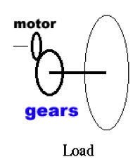
DC motor is a common actuator in control systems. It directly provides rotary motion and, coupled with wheels or a rack-and-pinion mechanism, can provide transitional motion. The picture to the left in Figure 1‑12 shows a large industrial DC motor; in control systems applications you’re more likely to see a small, lightweight, high-precision geared DC motor, like the one shown on the right. However, their system equations follow the same laws of physics.
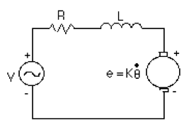
The diagram in Figure 1‑13 is a representation of the DC armature controlled motor, showing the electric circuit of the armature as well as mechanical parts of the motor, including gears. Small DC motors, such as the one driving the Servo Module in the lab, work most efficiently at high speeds, and therefore they have to be geared for most applications. Direct drives are found in some DC motors with large ratings. Motor equations are shown in Table 1‑6.
In the equations, R and L represent the resistance and inductance of the armature winding, [latex]K_t,K_e[/latex] represent the torque constant and the CEMF constant, respectively, n is the gear ratio and [latex]J_{eq},B_{eq}[/latex] represent the equivalent inertia and viscous friction coefficients of the motor and load combined, as reflected onto the motor side of the gear. Based on the above equations, a block diagram of the DC motor can be built, and is shown in Figure 1‑14.

 |
Armateur Winding:
[latex]v_{a} - v_{e} = Ri + L\frac{di}{dt}[/latex] Counter-electromotive (CEMF) force: [latex]v_{e} = K_{e}\omega[/latex] |
 |
Energy Conversion: [latex]T=K_{t}i[/latex]
[latex]J_{eq}\dot{\omega}_{m}=T-B_{eq}\omega_{m}[/latex] [latex]\omega=\dot{\theta}[/latex] |
 |
[latex]P_{motor} = P_{load}[/latex]
[latex]T_{m}\omega_{m} = T_{L}\omega_{L}[/latex] [latex]\frac{T_{m}}{T_{L}}=\frac{\omega_{L}}{\omega_{m}}=\frac{1}{n}[/latex] |
[latex]J_{m}\dot{w}_{m} + (J_{L}\dot{\omega}_{L})\cdot \frac{1}{n}=T -B_{m}\omega_{m}-(B_{L}\omega_{L})\cdot\frac{1}{n}[/latex]
[latex]J_{eq} = J_{m}+\frac{J_{L}}{n^{2}}[/latex] [latex]B_{eq} = B_{m} + \frac{B_{L}}{n^{2}}[/latex] |
The DC motor transfer function, [latex]G_m(s)[/latex], defined as the dynamic ratio of the load position output signal and the armature voltage input signal, is next derived from the above blocks, as shown below:
| [latex]G_{m}(s) = \frac{\frac{K_{t}}{(sL+R)(sJ_{eq}+B_{eq})}}{1+\frac{K_{t}K_{e}}{(sL+R)(sJ_{eq}+B_{eq})}}\cdot\frac{1}{n}\cdot\frac{1}{s}=\frac{K_{t}}{s^{2}LJ_{eq}+s(RJ_{eq}+LB_{eq})+RB_{eq}+K_{t}K_{e}}\cdot\frac{1}{n}\cdot\frac{1}{s}[/latex] | Equation 1‑16 |


This is a 3rd order transfer function. For small inductances L (or, L/R << J/B), this can be simplified:
| [latex]G_{m}(s) \approx \frac{K_{t}}{sRJ_{eq} + RB_{eq} + K_{t}K_{e}}\cdot\frac{1}{n}\cdot\frac{1}{s}[/latex] |
Equation 1‑17 |
Motor dynamics can now be approximated by a 2nd order transfer function. Two motor parameters are defined: [latex]K_{m}[/latex], called the motor gain constant, and [latex]\tau_{m}[/latex], called the motor time constant.
| [latex]K_{m} = \frac{K_{t}}{RB+K_{t}K_{e}}[/latex], [latex]\tau_m=\frac{RJ}{RB+K_{t}K_{e}}[/latex] |
Equation 1‑18 |
The motor transfer function can be written as:
| [latex]G_{m}(s) = \frac{K_{m}}{s\tau_{m}+1}\cdot\frac{1}{n}\cdot\frac{1}{s}[/latex] |
Equation 1‑19 |
The block diagram of motor representation shown in Figure 1‑14 can now be simplified to the one in Figure 1‑15:

How accurate is this approximation? Closed loop responses of the accurate servo module model and the model using a 2nd order approximation for the DC motor are shown in Figure 1‑16 – the responses are practically identical.

1.5.5 Examples
1.5.5.1 Example
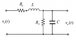
Consider a 2nd order filter, with a schematic as shown below:

Find the transfer function for this filter, if [latex]V_i[/latex]is an input to the system and [latex]V_o[/latex] is an output and the component values are [latex]R_{1}=10\Omega, R_{2}=5\Omega , L=2H,[/latex] and [latex]C=0.5F[/latex]. What kind of filter is this?
1.5.5.2 Example
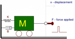
Consider a mechanical system shown in the following diagram. Derive the transfer function of this system with Force as an input signal and linear displacement as an output signal. Use MATLAB to simulate system responses for values of mass M = 1, spring flexibility K = 2 and friction B adjustable. Assume the force input to be in a form of an impulse or a very short pulse. Also, check the “Mass & Spring” animation/simulation in Matlab Demos.
1.5.5.3 Example
Consider the electric circuit below. Find its mechanical analog.

1.5.5.4 Example
Consider an electric circuit, a two-port, shown below, where its components have the following values: [latex]R_{1}=5\Omega, R_{2}=5\Omega, C=0.05F,[/latex] and [latex]L=0.1H.[/latex]
Find the transfer function of the two-port, [latex]G(s) = \frac{V_{o}(s)}{V_{i}(s)}[/latex]. Next, find an analytical expression for the two-port step response, [latex]v_{o}(t), t \geq 0[/latex].
