
Chapter 8
8.7 Examples
8.7.1 Example
Consider a closed loop system with the DC gain of 0.8 and the following closed loop pole locations: [latex]p_1 = -25[/latex], [latex]p_2=-1-j5.9161[/latex], [latex]p_3 = -1 + j5.9161[/latex]. Decide if a reduced order model is appropriate for this system.
8.7.2 Example
A certain LTI system is described as having four poles and one zero, as follows: [latex]p_1 = -1[/latex], [latex]p_2 = -1 - j1[/latex], [latex]p_3 = -10[/latex], [latex]p_4 = -2[/latex], [latex]z_1 = -2.2[/latex]. It is also recorded that the system has a DC gain of 5. Write the complete transfer function of the system in a ZPK form. Note the multiplier gain K in the ZPK form is NOT the same as the DC gain! Is it appropriate to use a simplified, 2nd order representation for this system? If so, please write the second order transfer function of this model, as well as its parameters (i.e. [latex]K_{dc}[/latex], [latex]\omega_n[/latex], [latex]\zeta[/latex]).
8.7.3 Example
Consider a transfer function of a certain industrial process, described as follows:
[latex]G(s)=\frac{50(s+4)(s^2+38s+364)(s+30)}{(s+3.95)(s+25)(s^2+7s+64)(s^2+40s+404)}[/latex]
Can a second order dominant poles model be used to represent this process? If so, explain why by sketching below a pole-zero map of G(s). Next, calculate the appropriate model parameters [latex]\zeta[/latex], [latex]\omega_n[/latex], and [latex]K_{dc}[/latex] and then write the transfer function of the model, [latex]G_m(s)[/latex].
8.7.4 Example
Consider a control system as shown:

When the Proportional Controller gain is K = 33, the closed loop system has the following poles: -7.1164, -4.4199, [latex]-0.2319\pm j2.0354[/latex] and a zero at -4. Briefly discuss if it is appropriate to model the closed loop system behaviour by using the standard second order system, and if so, derive the model parameters and write its transfer function [latex]G_m(s)[/latex].
NOTE: This example can be easily solved with access to Matlab. However, given the information provided, it can also be solved without any complicated polynomial manipulations. Use Matlab to check on your results.
8.7.5 Example
Consider the two responses shown. One is the response of a third order closed loop system with a dominant pair of complex poles and an additional real pole, the other is the response of a second order model based on the dominant pair of system poles. Match the responses with the plots.

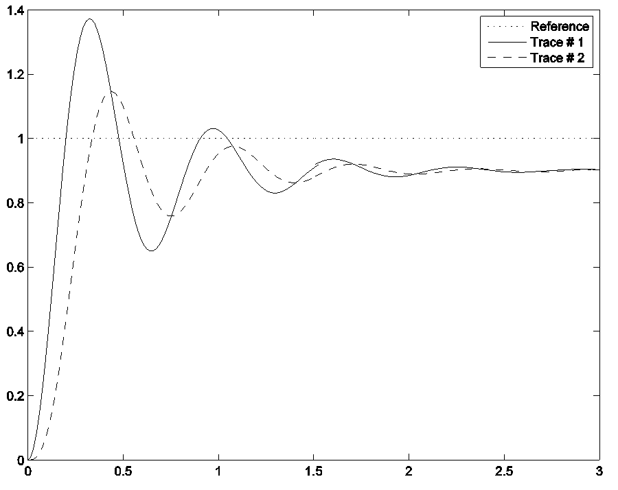
8.7.6 Example
Consider the three figures on the following page – each shows two responses, to a unit reference signal, of two closed loop control systems. One response, identical in each figure, is of a second order system with two complex conjugate poles. The second response in each figure has the same two complex conjugate poles and an additional singularity, i.e. either a pole or a zero. For each of the figures, finish the following sentence:
The second order system with two complex poles is trace # _______
Next, for each figure, choose which of the following answers applies to this case:
The other system has two complex poles and a significant real LHP pole
The other system has two complex poles and a significant real LHP zero
The other system has two complex poles and a significant real RHP pole
The other system has two complex poles and a significant real RHP zero
Figure A.
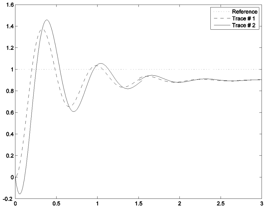
Figure B.
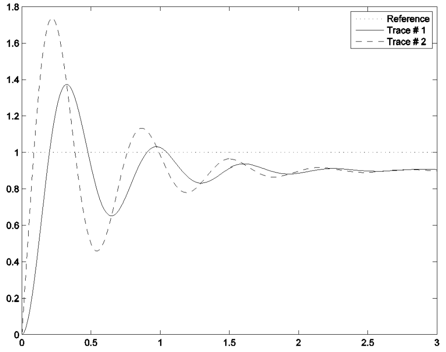
Figure C.
8.7.7 Example
Consider a certain closed loop control system, which is TYPE ONE. It is a second order system with two complex conjugate poles located at: [latex]-3 \pm j3[/latex]. Write its transfer function.
Consider a certain closed loop control system, which is TYPE ONE. It is a second order system with two complex conjugate poles located at: [latex]-3\pm j3[/latex] and a zero at -15. Write its transfer function.
Consider a certain closed loop control system, which is TYPE ONE. It is a second order system with two complex conjugate poles located at: [latex]-3 \pm j3[/latex] and a zero at +15. Write its transfer function.
Consider a certain closed loop control system, which is TYPE ONE. It is a third order system with two complex conjugate poles located at: [latex]-3 \pm j3[/latex] and a pole at -15. Write its transfer function.
8.7.8 Example
Consider a step response of a system as shown below. Choose which system description matches this response:
- Two complex poles at: -1–j4.9, -1 +j4.9 and gain K = 5;
- Two complex poles at: -1–j4.9, -1 +j4.9, zero at -5 and gain K = 5
- Two complex poles at: -1–j4.9, -1 +j4.9, zero at -5 and gain K = -5
- Two complex poles at: -1–j4.9, -1 +j4.9, zero at +5 and gain K = 5
- Two complex poles at: -1–j4.9, -1 +j4.9, zero at +5 and gain K = -5

8.7.9 Example
Consider a certain closed loop control system under Proportional Control, as shown.

Assume the Controller gain to be [latex]K_p = 3[/latex], calculate a transfer function of the closed loop system and determine the closed loop system damping ratio, [latex]\zeta[/latex], the closed loop frequency of natural oscillations, [latex]\omega_n[/latex] and the closed loop DC gain, [latex]K_{dc}[/latex]. Estimate the closed loop system transient and steady state response specifications.
Next, replace the Proportional Controller with a Lead Control as shown and find values of the controller parameters, [latex]a_1[/latex], [latex]a_0[/latex], [latex]b_1[/latex] such that the closed loop system has a dominant pair of complex poles with the frequency of damped oscillations equal to 2 rad/sec, and the corresponding time constant of 1 second, and a third real pole with the corresponding time constant of 0.05 seconds.

Find the closed loop transfer function of the compensated system, [latex]G_{cl}(s)=\frac{Y(s)}{R(s)}[/latex] and estimate the transient and steady state response specifications for the compensated system.
Consider step response plots shown next. One of the responses shown is the response of the system compensated according to instructions above, i.e. [latex]G_{cl}(s)[/latex], while the other one is the response of the system described by:
[latex]G_1(s)=\frac{100}{(s+20)(s^2+2s+5)}[/latex]
Label the two traces on the plot (i.e. Trace A and Trace B), by indicating which trace corresponds to which transfer function. Provide a brief explanation of why that is.

8.7.10 Example
Consider a certain closed loop control system which is supposed to work under the so-called Lead Controller:

Find values of the controller parameters, [latex]a_1[/latex], [latex]a_0[/latex], [latex]b_1[/latex] such that the closed loop system has a dominant pair of complex poles with the frequency of damped oscillations equal to 9 rad/sec, and the corresponding time constant of 0.5 seconds, and a third real pole with the corresponding time constant of 25 milliseconds. Find the closed loop transfer function of the compensated system, [latex]G_{cl}(s)=\frac{Y(s)}{R(s)}[/latex]. Next, consider the two step response plots shown below. One of the responses shown is the response of the system compensated according to instructions above, i.e. [latex]G_{cl}(s)[/latex], while the other one is the response of the system described by the transfer function [latex]G_1(s)[/latex], described below.
[latex]G_1(s)=\frac{3400}{(s+40)(s^2+4s+85)}=\frac{3400}{s^3+44s^2+245s+3400}[/latex]
Label the two traces on the plot (i.e. Trace A and Trace B), by indicating which trace corresponds to which transfer function. Provide a brief explanation of why that is. Finally, consider now two step response plots shown next. One of them corresponds to the Lead compensated closed loop system that has three poles and one zero, and the other corresponds to a system described by a second order model by the transfer function [latex]G_2(s)[/latex] below that has only two poles. Explain briefly why this model fits the compensated system so well.
[latex]G_2(s)=\frac{85}{s^2+4s+85}[/latex]

8.7.11 Example
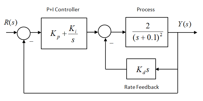
Consider the following block diagram, where a Proportional + Integral Controller is implemented in the forward path, with a Derivative Control implemented as a Rate Feedback in an inner feedback loop, as shown.

Derive the closed loop transfer function, [latex]G_{cl}(s)=\frac{Y(s)}{R(s)}[/latex], in terms of the controller parameters, [latex]K_p[/latex], [latex]T_i[/latex] and [latex]T_d[/latex]. It is desired that the closed loop system step response has a zero steady state error, percent overshoot of 15% and the settling time (±2% criterion) of 1 second. Use the “top-down” design to find appropriate controller parameters.
HINT: Assume that has the closed loop system has two dominant poles with a damping ratio [latex]\zeta[/latex] and the natural frequency [latex]\omega_n[/latex] corresponding to the desired step response specification, and that the third closed loop pole is at a location ten (10) times further to the left of the s-plane than the Real Part of the dominant poles pair.
Once you design your controller, discuss whether the system response is going to be exactly as expected. If not, explain why, and what the differences might be.
8.7.12 Example
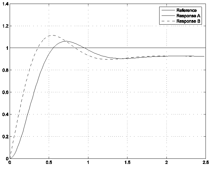
Consider again the block diagram in Example 7.3.20, describing a certain control system where a Proportional + Rate Feedback control is implemented with two gains [latex]K_p[/latex] and [latex]K_d[/latex]. Replace the P + Rate Feedback Control with PD Control, using the same gain values as in Example 7.3.20:
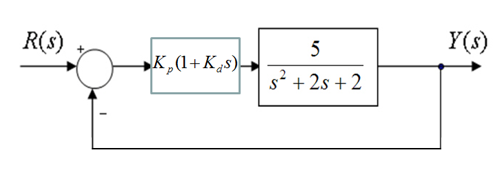
Given the two responses shown next, which one corresponds to the system under P + Rate Feedback, and which one to the system under PD Control?
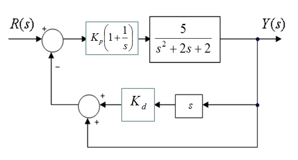
Assume now that the proportional gain in Example 7.3.20 has been replaced by a P+I controller with the transfer function [latex]K_p(\frac{1}{s} +1)[/latex], while the Rate Feedback gain remains as in Example 7.3.20. Briefly discuss what the effect of this new controller will have on the system response, in terms of its steady state error, percent overshoot, and rise time.
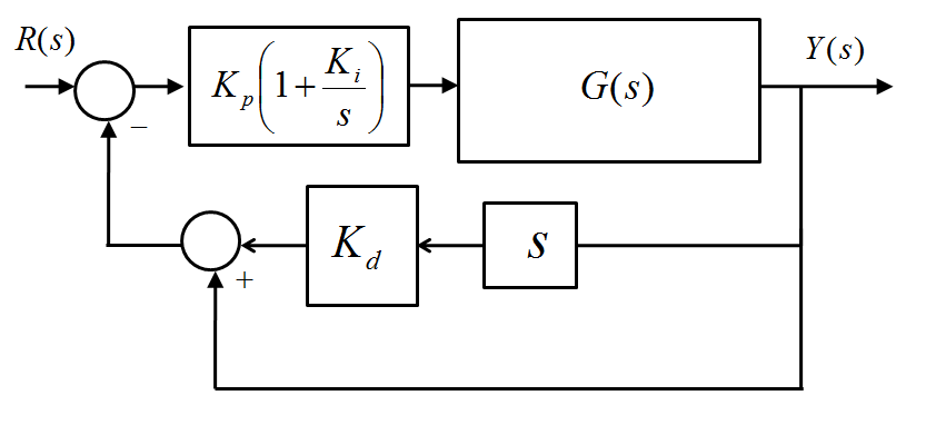
8.7.13 Example
Consider the same block diagram as in the previous two examples, describing a certain control system where a Proportional + Rate Feedback control is implemented with two gains [latex]K_p[/latex] and [latex]K_d[/latex]. Recall that the conclusion in the first example was that the Proportional + Rate Feedback control can meet exactly either the specifications for the Percent Overshoot and the Settling Time, or for the Percent Overshoot and the Steady State Error, but not for all three. Now, add the Integral term in series with the Proportional Gain, as shown in the diagram in the second example, and see if the exact values of the required PO, the required Settling Time and the required Steady State Error can be met: PO = 15% , [latex]T_{settle(\pm 2\%)} = 1.5[/latex] seconds and [latex]e_{ss(step)\%} = 0[/latex].
8.7.14 Example
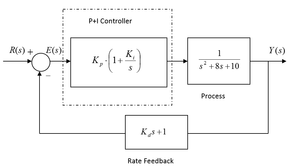
Consider again the system from Example 7.3.17, describing a certain system under Proportional + Rate Feedback Control. We found the closed loop system transfer function for this system in terms of controller gains [latex]K_p[/latex] and [latex]K_d[/latex] and we determined values of the controller gains such that PO = 10% and Settling time (within [latex]\pm2\%[/latex]) = 1 second. These gain values were: [latex]K_p = 40.78[/latex] and [latex]K_d = 0.0245[/latex].
Now, let’s consider a modified version of this system, with the same process transfer function G(s), but now the closed loop position control system works under Proportional + Integral + Rate Feedback Control, as shown next.
Find the closed loop system transfer function in terms of controller gains [latex]K_p[/latex] and [latex]K_d[/latex] and [latex]K_i[/latex]. Rewrite this transfer function using values of gains [latex]K_p[/latex] and [latex]K_d[/latex] as calculated in Example 7.3.17 so that your transfer function will only have one variable gain, [latex]K_i[/latex].
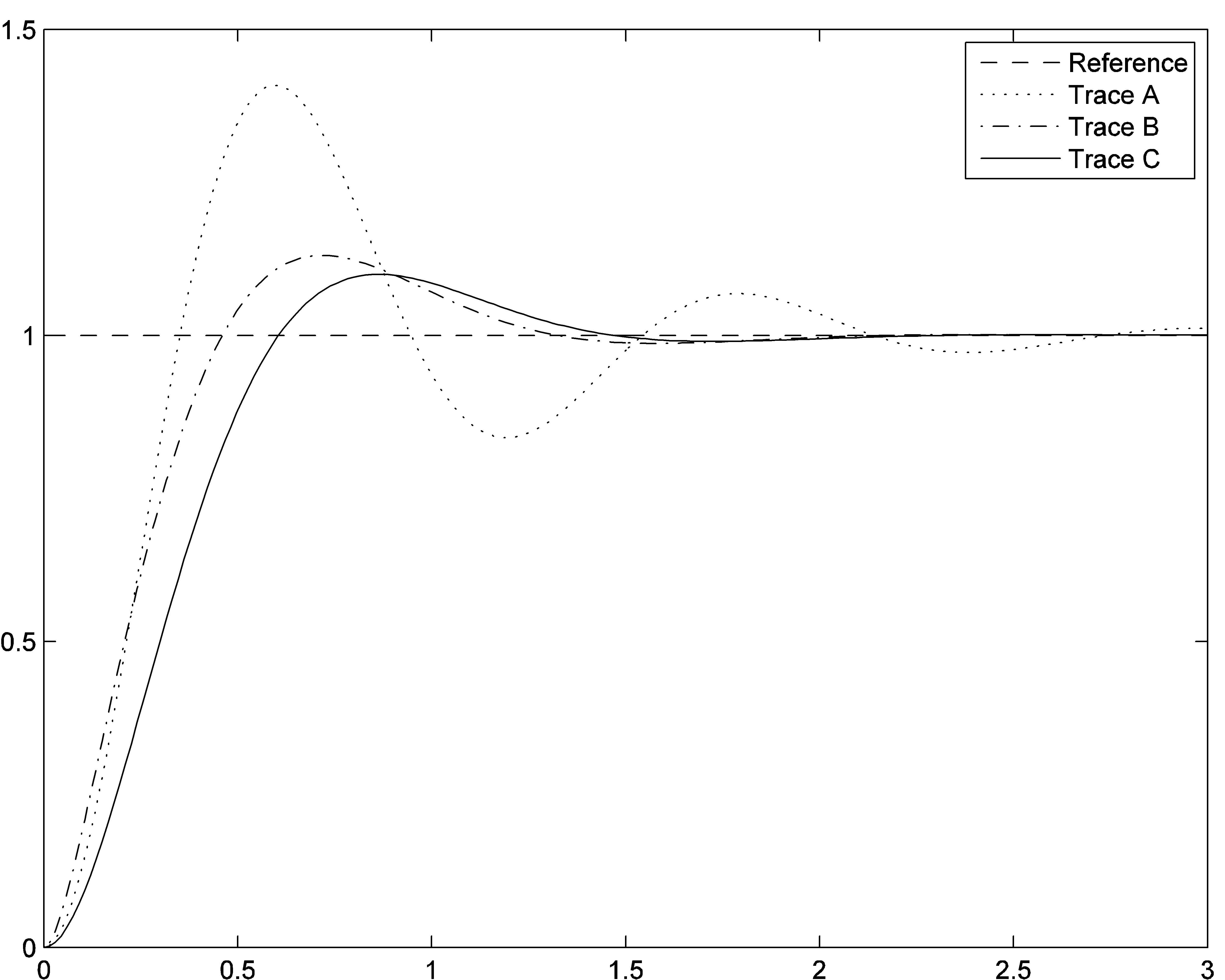
Next, consider the following three transfer functions [latex]G_1(s)[/latex], [latex]G_2(s)[/latex] and [latex]G_3(s)[/latex] that correspond to three specific values of the Integrator gain [latex]K_i[/latex]:
[latex]G_1(s)=\frac{40.78(s+0.3)}{(s+0.28)(s^2+7.72s+43.93)}[/latex]
[latex]G_2(s)=\frac{40.78(s+0.7)}{(s+0.69)(s^2+7.31s+41.45)}[/latex]
[latex]G_3(s)=\frac{40.78(s+02)}{(s+2.37)(s^2+5.63s+34.45)}[/latex]
The graph below shows the step responses to a unit reference of the three transfer functions:
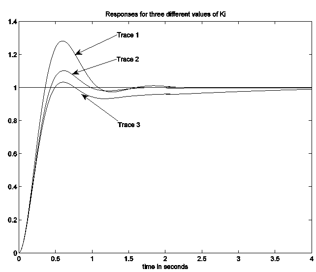
Identify the numerical value of the Integrator gain that corresponds to each transfer function and then match it with one of the three traces shown in the plot. How did you match plots with transfer functions and gain values? Explain briefly.
If the P+Rate Feedback Controller from Example 7.3.17 and one of the PI+Rate Feedback Controllers in this example both meet these specs: PO = 10% and Settling time (within [latex]\pm2\%[/latex]) = 1 second, is PI+Rate a better controller? If yes, briefly explain why? If no, briefly explain why.
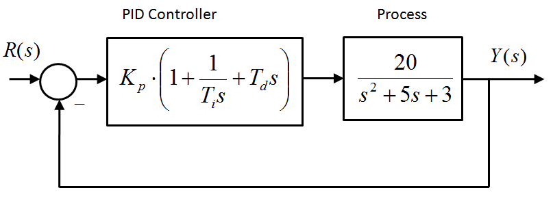
8.7.15 Example
Consider a feedback system under PID Control as shown. Your task is to calculate the PID Controller parameters. To do so, please follow the steps described in the following parts.
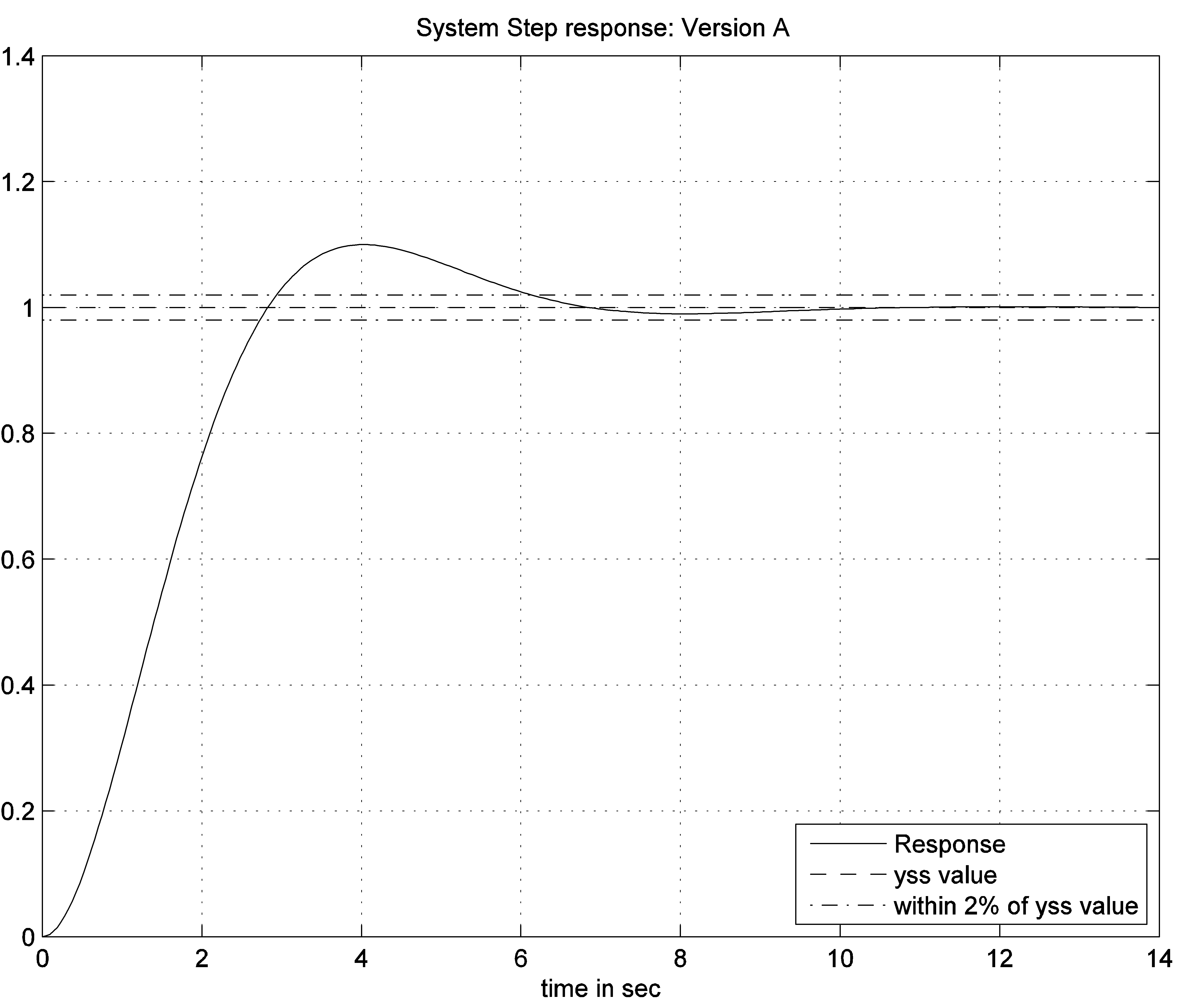
We want the compensated closed loop response of our control system to resemble the response of a standard second order under-damped model that is shown below. Determine appropriate parameters of the model (i.e. [latex]K_{dc}[/latex], [latex]\omega_n[/latex], [latex]\zeta[/latex]). Write the parameters as well as the model transfer function.
Derive the closed loop transfer function, [latex]G_{cl}(s)=\frac{Y(s)}{R(s)}[/latex], in terms of the controller parameters, [latex]K_p[/latex], [latex]T_i[/latex], and [latex]T_d[/latex]. Find appropriate controller parameters. HINT: Assume the dominant poles model for the closed loop system based on the model derived in Part 1 and use a factor of 10 times for any additional poles to be placed in the insignificant region. Substitute the computed values of the controller parameters, [latex]K_p[/latex], [latex]T_i[/latex], and [latex]T_d[/latex] into the closed loop transfer function, [latex]G_{cl}(s)=\frac{Y(s)}{R(s)}[/latex] and write the numerical values of its poles and zeros, as well as the DC Gain of the compensated closed loop. Sketch a Pole-Zero Map for this transfer function. Based on the Pole-Zero Map, discuss briefly whether the actual compensated system response will differ from the expected model response, and if so, describe in what way. Try to be brief but specific.
8.7.16 Example
Consider a closed loop positioning control system with a PID Controller in a so-called “series” configuration, as shown:
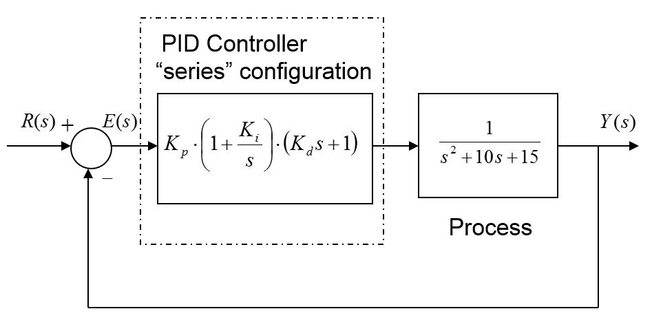
Derive the Closed Loop system transfer function in terms of Controller Gains [latex]K_p[/latex], [latex]K_d[/latex], and [latex]K_i[/latex] and write the system Characteristic Equation, [latex]Q(s) =0[/latex]. The compensated Closed Loop step response of this system is to have the following specifications: [latex]PO=10\%[/latex] and [latex]T_{settle(\pm2\%)} = 0.9[/latex] sec. Determine the Closed Loop system damping ratio, [latex]\zeta[/latex], and the frequency of natural oscillations, [latex]\omega_n[/latex], to meet the transient response requirements.
Choose the pole locations for the Closed Loop system so that system two complex conjugate (“dominant”) poles correspond to the desired second order model (above) and the third real pole equals to the value of Integral Gain so that a pole-zero cancellation in the Closed Loop transfer function occurs. Compute the required Controller gains [latex]K_p[/latex], [latex]K_d[/latex] and [latex]K_i[/latex]. Note that you are expected to solve a quadratic equation to find the gains in item 3), which means you will have two sets of solutions. Choose ONLY ONE set for your final answer – clearly identify it, and justify your choice by briefly commenting on any possible differences between the expected system responses (i.e. of the dominant poles model) and the actual system responses.
8.7.17 Example
Consider again the same configuration as in Example 8.7.16, where the transfer function of the process is:
[latex]G(s)=\frac{1}{s^2+7s+8}[/latex]
The compensated Closed Loop step response of this system is to have the following specifications: [latex]PO=15\%[/latex] and [latex]T_{settle(\pm2\%)} = 2[/latex] sec. Determine the Closed Loop system damping ratio, [latex]\zeta[/latex], and the frequency of natural oscillations, [latex]\omega_n[/latex], to meet the transient response requirements.
Choose the pole locations for the Closed Loop system so that system two complex conjugate (“dominant”) poles correspond to the desired second order model (above) and the third real pole equals to the value of Integral Gain [latex]K_i[/latex] so that a pole-zero cancellation in the Closed Loop transfer function occurs. Compute the required Controller gains [latex]K_p[/latex], [latex]K_d[/latex], and [latex]K_i[/latex]. Note that you are expected to solve a quadratic equation to find the gains in item 3), which means you will have two sets of solutions. Choose ONLY ONE set for your final answer – clearly identify it, and justify your choice by briefly commenting on any possible differences between the expected system responses (i.e. of the dominant poles model) and the actual system responses. Suggest possible improvements.
8.7.18 Example
Consider a closed loop positioning system working under Proportional + Integral + Rate Feedback Control, as shown below.
Derive the Closed Loop system transfer function in terms of Controller Gains [latex]K_p[/latex], [latex]K_d[/latex], and [latex]K_i[/latex] and write the system Characteristic Equation, [latex]Q(s)=0[/latex]. Next, the compensated Closed Loop step response of this system is to have the following specifications: [latex]PO=10\%[/latex] and [latex]T_{settle(\pm2\%)} = 1[/latex] sec. Determine the Closed Loop system damping ratio, [latex]\zeta[/latex], and the frequency of natural oscillations, [latex]\omega_n[/latex], to meet the transient response requirements.
Next, choose the pole locations for the Closed Loop system so that system two complex conjugate (“dominant”) poles correspond to the desired second order model (above) and the third real pole equals to the value of Integral Gain so that a pole-zero cancellation in the Closed Loop transfer function occurs. Compute the required Controller Gains [latex]K_p[/latex], [latex]K_d[/latex], and [latex]K_i[/latex]. Note that you are expected to solve a quadratic equation to find the gains in item 3), which means you will have two sets of solutions. Choose ONLY ONE set for your final answer – clearly identify it, and briefly justify your choice.
8.7.19 Example
Consider a closed loop unit feedback control system with a process transfer function as follows:
[latex]G(s)=\frac{2}{s^2(s+10)}[/latex]
The system is to work either under a Proportional + Derivative (PD) Control or under a Proportional + Rate Feedback, both shown next. The closed loop transfer functions of both systems are already derived in terms of Controller parameters [latex]K_p[/latex] and [latex]T_d[/latex], and shown.
The closed loop transfer function of the system under PD Control can be derived as follows:
[latex]G_{cl1}(s)=\frac{2K_p (T_d s +1)}{s^3+10s^2+2K_pT_ds+2K_p}[/latex]
The closed loop transfer function of the system under P + Rate Feedback Control Control can be derived as follows:
[latex]G_{cl2}(s)=\frac{2K_p}{s^3+10s^2+2K_pT_ds+2K_p}[/latex]
We would like the closed loop transfer function to resemble a second order model with the following parameters: DC Gain, , the damping ratio, , and the frequency of natural oscillations, . The model is described by the transfer function below:
[latex]G_{m}(s)=K_{dc}\frac{\omega_n^2}{s^2+2\zeta\omega_ns+\omega_n^2}[/latex]
In order for that to be true, any additional poles and zeros of the closed loop would have to be placed in the “insignificant region” of the S-plane. Show why it is not possible to implement a PD Controller with a third closed loop pole at the exact location of [latex]-\frac{1}{T_d}[/latex] so that a perfect pole-zero cancellation in the closed loop transfer function [latex]G_{cl1}(s)[/latex] could take place. Next, consider that the closed loop step response is to have a Percent Overshoot of 10% and the Settling Time ([latex]T_{settle(\pm2\%)}[/latex]) equal to 0.8 seconds. Show why it is not possible to implement a P + Rate Controller where we would have the dominant complex poles so that the above specs are met, and a third closed loop pole at the location that is 10 times further to the left of the S-plane than the location of the dominant complex poles, i.e. in the insignificant region.
While it is not possible to have all three conditions from Part 2 met, it is possible to find the P + Rate Controller parameters [latex]K_p[/latex] and [latex]T_d[/latex] such that the PO = 10%, and the third pole of the closed loop system is 10 times further to the left of the S-plane than the location of the dominant complex poles, i.e. in the insignificant region. Compute the Controller parameters [latex]K_p[/latex] and [latex]T_d[/latex], then find the resulting natural frequency and estimate the resulting Settling Time ([latex]T_{settle(\pm2\%)}[/latex]) of the compensated closed loop step response.
8.7.20 Example
Consider a closed loop control system working in a feedback configuration under Proportional + Rate Feedback Control, shown in Figure below:
Determine the value of the Proportional Gain, [latex]K_p[/latex], such that the closed loop step response will have a Steady State Error of 5%. Next, determine an APPROXIMATE value of the Rate Feedback Gain, [latex]K_d[/latex], such that the closed loop step response will have a Percent Overshoot of 15%. HINT: Make a simplifying assumption based on the Dominant Poles Model to arrive at this estimate.
Next, determine the ACCURATE value of the Rate Feedback Gain, [latex]K_d[/latex], such that the closed loop step response will have a Percent Overshoot of 15%. Note that you are solving only a quadratic equation. Finally, compare the two values of the Rate Feedback Gain, [latex]K_d[/latex], (i.e. the approximate and the accurate value) and comment on whether the simplifying assumption you made in the previous item is valid, and on how much difference, if any, using the approximate value would make. You may want to refer to the pole-zero map of the compensated closed loop system to make your argument.
8.7.21 Example
Consider a unit feedback control system where the process is a first order transfer function G(s), and the Controller transfer function is described below as [latex]G_c(s)[/latex]:
[latex]G(s)=\frac{1}{(s+0.5)}[/latex]
[latex]G(s)=\frac{a_1s+a_0}{b_1s+1}[/latex]
Derive the closed loop transfer function, [latex]G_{cl}(s)=\frac{Y(s)}{R(s)}[/latex], in terms of the controller parameters, [latex]a_1[/latex], [latex]a_0[/latex], and [latex]b_1[/latex], and write the system Characteristic Equation, [latex]Q(s)=0[/latex].
Assume that the closed loop system response can be approximated using a second order dominant poles model. The compensated closed loop step response of this system is to have the following specifications: Percent Overshoot, [latex]PO=10\%[/latex], Settling Time, [latex]T_{settle(\pm2\%)} = 2[/latex] sec, and Steady State Error, [latex]e_{ss(\%)} = 5\%[/latex]. Identify an appropriate model, [latex]G_m(s)[/latex], that would meet these specifications.
Next, find controller parameters ([latex]a_1[/latex], [latex]a_0[/latex], and [latex]b_1[/latex]) and identify the nature of the controller i.e. is it a PD, PI, PID, Lead or Lag Controller.
Briefly describe how the actual closed loop system response would compare with the model response.
8.7.22 Example
Consider the closed loop control system with a relatively slow hydraulic process under a modified PID Control, with Rate Feedback replacing the Derivative term, as shown in the diagram next.
The desired step response specifications are as follows:
- Percent Overshoot, [latex]PO=20\%[/latex]
- Settling time within 2% of the steady state value, [latex]T_{settle(\pm2\%)} = 10[/latex] seconds
- Steady State Error, [latex]e_{ss\%} = 0[/latex]
Your task is to calculate the PID Controller parameters, [latex]K_p[/latex], [latex]K_d[/latex], and [latex]K_i[/latex] so that the above specifications are met. In order to do so, follow the steps outlined next.
Find the closed loop transfer function, [latex]G_{cl}(s)[/latex], in terms of controller gains [latex]K_p[/latex], [latex]K_d[/latex], and [latex]K_i[/latex]. Choose the location for the two dominant poles of the closed loop based on a standard second order dominant poles model. Compute model parameters [latex]\omega_n[/latex], [latex]\zeta[/latex], as appropriate, given the time response specifications.
Find the controller gains [latex]K_p[/latex], [latex]K_d[/latex], and [latex]K_i[/latex] so that the design benefits from a pole-zero cancellation, thus resulting in a closed loop transfer function identical to that of the above model, i.e. [latex]G_{cl}(s)=G_m(s)[/latex]. HINT: This can be accomplished by placing the third closed loop pole at the EXACT location of the closed loop zeros from above. What is the resulting Steady State Error to a unit ramp reference signal?
Next, consider the same closed loop control system and the same transient requirements, but now it is also required that the compensated closed loop response tracks the unit ramp with the steady state error equal to 0.2 units (e_{ss(ramp)}=0.2). Check your calculations in item 4) to determine which controller gain is responsible for the steady state ramp error, and calculate the value of that gain so that the error condition is met.
Since the ramp steady state error will pre-determine one of the controller gains (see above), we can no longer impose the perfect pole-zero cancellation requirement on the design. Therefore, assume that the third closed loop pole is at location s = -a, which needs to be determined, together with the two remaining controller gains. Find the value of as well as of the two gains. The first design uses a pole-zero cancellation so its response is expected to be exactly like the response of a second order system. Check off in the tables below how different the response of the second design is, based on where its poles and zeros are and briefly explain why?
| Higher? | Lower? | The Same? | |
| Percent Overshoot | |||
| Rise Time | |||
| Steady State Error for a step reference | |||
| Steady State Error for a ramp reference |
8.7.23 Example
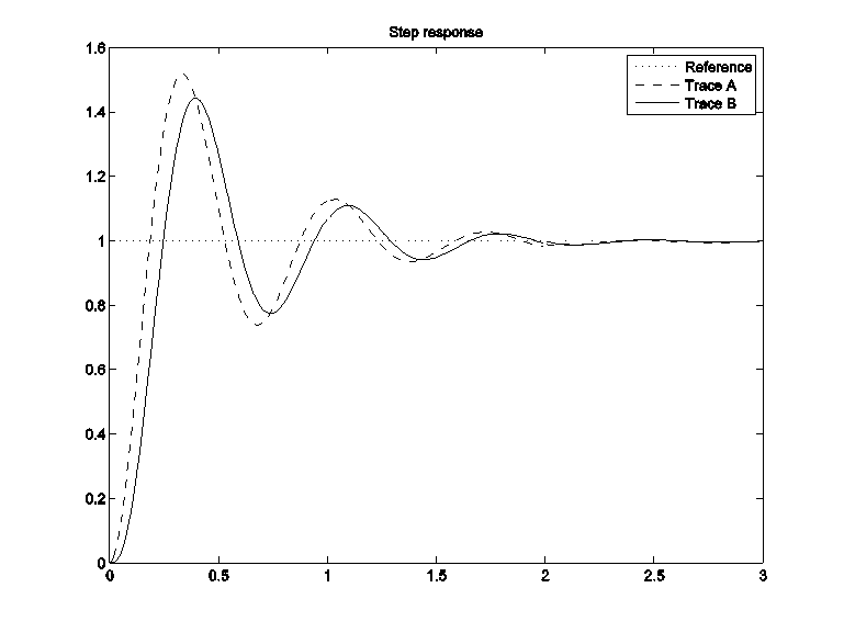
Consider again a unit feedback closed loop control system from Example 8.7.10, where the process transfer function was described below as G(s), and the Controller transfer function [latex]G_c(s)[/latex] was a Lead Controller.
[latex]G(s)=\frac{30}{s(s+3)}[/latex] [latex]G(s)=\frac{a_1s+a_0}{b_1s+1}[/latex]
Derive the closed loop transfer function, [latex]G_{cl}(s)=\frac{Y(s)}{R(s)}[/latex], in terms of the controller parameters, [latex]a_1[/latex], [latex]a_0[/latex], and [latex]b_1[/latex], identify the closed loop characteristic equation. It is required that the compensated closed loop step response of this system have the following specifications: Percent Overshoot, [latex]PO=15\%[/latex], Settling Time, [latex]T_{settle(\pm2\%)} = 1.5[/latex] sec, and Steady State Error, [latex]e_{ss(\%)}=0\%[/latex]. Use the “Top-Down” design approach to identify the required closed loop characteristic equation that would meet the specifications, and find appropriate controller parameters, [latex]a_1[/latex], [latex]a_0[/latex], and [latex]b_1[/latex]. Write the required closed loop characteristic equation, controller parameters and its transfer function, [latex]G_c(s)[/latex], and identify the nature of the controller (i.e. is it PD, PI, PID, Lead or Lag Controller).
HINT: Assume that has the closed loop system has two dominant poles with a damping ratio [latex]\zeta[/latex] and the natural frequency [latex]\omega_n[/latex] corresponding to the desired step response specification, and that the third closed loop pole is at a location ten (10) times further to the left of the s-plane than the Real Part of the dominant complex poles.
The next figure shows a comparison of the step responses to a unit reference – these are the uncompensated closed loop step response, compensated closed loop step response and 2nd order dominant pair model step response. Identify the traces on the plot, i.e. match each trace label with the correct description.
8.7.24 Example
Consider again the positioning system from Example 3.3.13, shown next. The transfer functions [latex]G_{cl}(s)[/latex] and [latex]G_d(s)[/latex] were derived and the numerical values substituted:
[latex]G_{cl}(s)=\frac{\Omega(s)}{\Omega_{ref}(s)}=\frac{80}{s^2+21.4s+188}[/latex] [latex]G_{cl}(s)=\frac{\Omega(s)}{T_{dist}(s)}=\frac{-0.02s-40}{s^2+21.4s+188}[/latex]
The system output was: [latex]\Omega(s)=G_{cl}(s)\cdot R(s)+G_d(s)\cdot T_{dist}(s)[/latex]. For the resulting system transfer function [latex]G_{cl}(s)[/latex], estimate the following closed loop step response specifications: [latex]e_{ss(step)\%}[/latex] – steady step error in % to a normalized unit step input, P.O. – Percent Overshoot, and [latex]T_{settle(\pm2\%)}[/latex] – settling time.
Next, assume K = 1; if the reference speed signal is [latex]\omega_{ref}(t)=300\frac{rad}{sec}[/latex] and [latex]T_{dist}(t)=0[/latex], what is the output speed? With the same reference, if the torque disturbance signal is [latex]T_{dist}(t)=100Nm[/latex], what is the output speed change in [latex]\frac{rad}{sec}[/latex]?
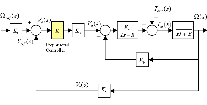
Next, calculate the required Proportional Gain K to achieve [latex]e_{ss(step)\%}=10\%[/latex]. For that value of K, estimate the resulting P.O. and [latex]T_{settle(\pm2\%)}[/latex]. If the reference speed signal is [latex]\omega_{ref}(t)=300\frac{rad}{sec}[/latex] and [latex]T_{dist}(t)=0[/latex], what is the output speed? With the same reference and gain K, if the torque disturbance signal is [latex]T_{dist}(t)=100Nm[/latex], what is the output speed change in [latex]\frac{rad}{sec}[/latex]?
