3.1 Basic Block Diagrams Continued

Recall the Basic Block Diagram operations from Chapter 1.6: blocks in series, blocks in parallel, and a basic closed loop. These simple rules of Block Diagram simplifications are not always sufficient. For example, consider the block diagram below:

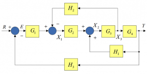
In order to calculate the system transfer function, [latex]G(s) = \frac{Y(s)}{R(s)}[/latex], we need to look at some other rules, as follows.

3.1.1 Moving the Summer in Front of a Block

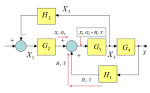
Consider the segment of the block diagram in Figure 3‑1, shown in Figure 3‑2. It cannot be “collapsed” using the closed loop formula, or a series of blocks formula, or a parallel blocks formula. Pay attention to the signal in a blue frame. The feedback signal [latex]H_{1} \cdot Y[/latex] connects to the “inner summer” where it is added to the signal [latex]X_{1} \cdot G_{2}[/latex]. The signal in the blue frame is an output of the “inner summer”, and therefore it is equal to. The signal in the blue frame is an output of the “inner summer”, and therefore it is equal to [latex]X_{1} \cdot G_{2} + H_{1} \cdot Y[/latex].

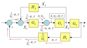
Consider now the same segment of the block diagram, but with a small modification as shown in Figure 3‑3. The “inner summer” is moved in front of block [latex]G_{2}[/latex] – to maintain the signal equivalency, the feedback signal [latex]H_{1} \cdot Y[/latex] is now fed through block [latex]\frac{1}{G_{2}}[/latex]. Note how the signal [latex]H_{1} \cdot Y \cdot \frac{1}{G_{2}}[/latex] travels (red arrows) around the feedback loop and finally is fed through block [latex]G_{2}[/latex]– on the output of that block it is added to signal [latex]X_{1} \cdot G_{2}[/latex] and thus the signal in the box is still equal to [latex]X_{1} \cdot G_{2} + H_{1} \cdot Y[/latex]. The equivalency of signals has been maintained.

However, unlike the diagram above, its equivalent below can now easily be “collapsed”: blocks [latex]G_{2}[/latex] and [latex]G_{3}[/latex] can be replaced by their product, next the feedback loop formula can be applied to them [latex]H_{2}[/latex] with as feedback, the result can be put in series with block [latex]G_{4}[/latex] and finally, the feedback loop formula can be applied, with [latex]H_{1}  \cdot \frac{1}{G_{2}}[/latex] as feedback.

Note that if a summer were to be moved behind the block, the additional gain would be equal to the value of the block gain, instead of its inverse.

3.1.2 Moving the Take-off Point Behind a Block

Consider the same segment of the block diagram in our example, and focus on [latex]X_{3}[/latex] the signal, as shown in Figure 3‑4. Again, any adjustment must maintain the signal equivalency. Pay attention to the output of block [latex]G_{3}[/latex] – signal [latex]X_{3}[/latex] – it is also the signal entering block. Consider now the same segment of the block diagram, with a small modification, as shown in Figure 3‑5.

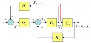
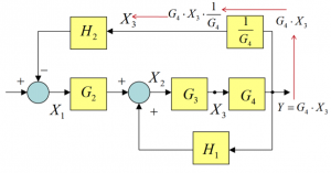
The take-off point is moved behind block [latex]G_{4}[/latex] and at the same time a block [latex]\frac{1}{G_{4}}[/latex] is placed in the path of the output signal [latex]Y = G_{4} \cdot X_{3}[/latex]. As a result, the signal being fed to block [latex]H_{2}[/latex] is still equal to [latex]X_{3}[/latex]. At this point, it is easy to see that blocks [latex]G_{3}[/latex] and [latex]G_{4}[/latex] can be replaced by their product, and then the feedback formula applied with [latex]H_{1}[/latex] as feedback, the result is put in series with block [latex]G_{2}[/latex] and again, the feedback formula can be applied, with [latex]H_{2} \cdot \frac{1}{G_{4}}[/latex] in feedback. Thus, the whole diagram can be successfully “collapsed”. Note that if a take-off point were to be moved in front of the block, the additional gain would be equal to the value of the block gain, instead of its inverse.

3.1.3 Summary

Moving the Summer behind the Block:

[latex](R(s) + X(s)) \cdot G_{1}(s) = R(s) \cdot G_{1}(s) + X(s) \cdot G_{1}(s)[/latex]

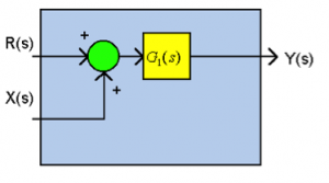
Moving the Summer in front of the Block:

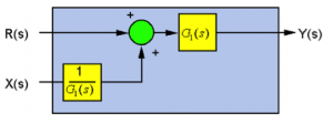
[latex]R(s) \cdot G_{1}(s) + X(s) = \bigg(R(s) + X(s) \cdot \frac{1}{G_{1}(s)} \bigg) \cdot G_{1}(s)[/latex]

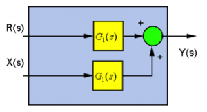
Moving the Take-off Point behind the Block:

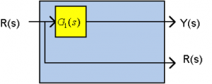
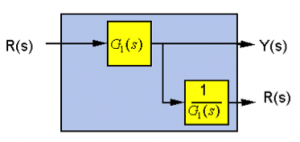
[latex]Y(s) = R(s) \cdot G_{1}(s)[/latex]

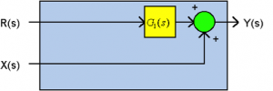
Moving the Take-off Point in front of the Block:

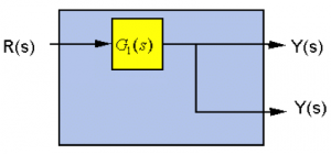
[latex]Y(s) = R(s) \cdot G_{1}(s)[/latex]

3.1.2 Example of Block Diagram

Let’s now go back to our example, shown in Figure 3‑1. Moving the take-off point behind the block, as shown in Figure 3‑5 results in a diagram configuration that can be easily “collapsed” using series and closed loop formula:

[latex]G = \frac{Y}{R} = \frac{G_{1}G_{2}G_{3}G_{4}}{1+G_{1}G_{2}G_{3}G_{4}H_{3} - G_{3}G_{4}H_{1} + G_{2}G_{3}H_{2}}[/latex]