3.3 Examples

3.3.1 Example

Consider a system described by the signal flow graph as shown below. Find its transfer function, [latex]G(s) =\frac{Y(s)}{U(s)}[/latex] , using the Mason’s Gain formula.

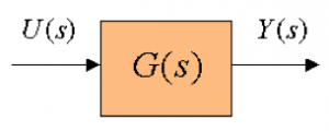
3.3.2 Example

Consider a system described by the signal flow graph as shown below. Find its transfer function, [latex](s) =\frac{Y(s)}{U(s)}[/latex] , using the Mason’s Gain formula.

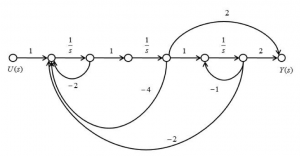
3.3.3 Example

Consider the transfer function shown and sketch a signal flow graph to represent it.

[latex]G(s) = \frac{s^{2} + 3s + 3}{s^{3} + 6s^{2} + 11s + 6}[/latex]

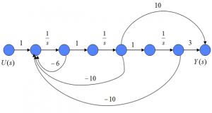
3.3.4 Example

Consider another similar example and find a signal flow graph representation for G(s) as shown, and sketch a signal flow graph to represent it.

[latex]G(s) = \frac{10s^{2}}{10s^{2} + 27s + 15}[/latex]

3.3.5 Example

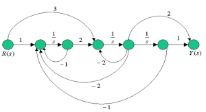
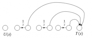
Consider the signal flow graph below. Apply the Mason’s Gain formula to obtain its transfer function. This is a difficult example. Expect 11 loops and 7 paths in the signal flow graph. Try to keep your loops and paths in an organized way – the suggestion is to number the nodes and write out the loops and the paths using the node numbers.

3.3.6 Example

Consider the signal flow graph below representing a system with two inputs. Apply the Mason’s Gain formula to determine both the system transfer function, here referred to as [latex]T_{1}(s) = \frac{Y(s)}{R(s)}[/latex]and the disturbance transfer function, which is referred to as [latex]T_{2}(s) = \frac{Y(s)}{D(s)}[/latex].

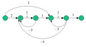
3.3.7 Example

Consider the signal flow graph below. Find the transfer function of the system. What is the system order? What is the system DC gain? What is the system’s high-frequency gain? What kind of a filter would that be?

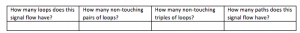
3.3.8 Example

Consider the signal flow graph shown. Complete the Table below, then find the system transfer function [latex]G(s) = \frac{Y(s)}{R(s)}[/latex].

3.3.9 Example

Consider the signal flow graph shown. Complete the Table below, then find the system transfer function [latex]G(s) = \frac{Y(s)}{R(s)}[/latex], write out the system characteristic equation and check if [latex]G(s)[/latex] is stable.

3.3.10 Example

Consider a signal flow graph as shown. Find the closed loop system transfer function. Show all loop and path gains, calculations for the cofactors, the main determinant of the signal flow graph, and the final transfer function of the system both in the polynomial ratio (TF) form, as well as in the pole-zero-gain (ZPK) form.

Compute the analytical system response to a unit step input.

3.3.11 Example

Consider again the servo-control system for a position control of the robot joint from Example 2.6.11, shown in Figure 2‑3. We found its transfer function using simple block diagram reduction. Now, do it using the Mason’s Gain formula.

3.3.12 Example

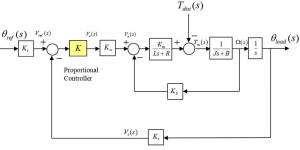
Consider yet again the servo-control system for a position control of the robot joint from Example 2.6.11, but now modified to allow for modelling of a disturbance and shown in Figure 3‑8. Find the transfer function between the disturbance torque [latex]T_{dist}[/latex] and the output load angle [latex]\Theta_{load}[/latex] :

[latex]G_{dist}(s) = \frac{\Theta_{load}(s)}{T_{dist}(s)}[/latex]

3.3.13 Example

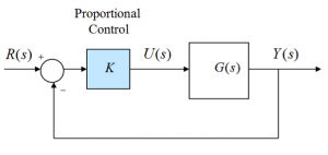
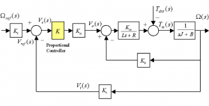
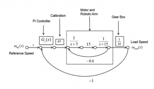
Now let’s consider a speed-control servomotor system under Proportional Control, as shown in the next figure, which is a variation on the previous servo-control configuration. Here, [latex]\omega_{ref}(t)[/latex] is the reference angular velocity signal, [latex]\omega (t)[/latex] is the actual angular velocity signal and [latex]T_{dist}[/latex] is a torque disturbance. This analog control system utilizes the same armature-controlled DC motor, but with a speed pickup arranged through a tachometer [latex]K_{t} = 0.2 \frac{v.sec}{rad}[/latex]. The remaining systems parameters are as in the previous servo-control examples: [latex]K_{a} = 10\frac{V}{V}[/latex] – amplifier gain, [latex]K_{m} = 2\frac{N.m}{A}[/latex] – motor torque constant, [latex]R = 2 \Omega[/latex] – armature resistance, [latex]L = 0.1H[/latex] – armature inductance, [latex]K_{b} = 2\frac{V \cdot sec}{rad}[/latex] – CEMF constant, [latex]J = 0.5\frac{N. m. sec^{2}}{rad}[/latex] – motor & load inertia, and [latex]B = 0.7\frac{N. m \cdot sec}{rad}[/latex] – motor & load linear friction coefficient.

Set the Proportional Gain K = 1, and use the Mason’s Gain formula to derive the closed loop system transfer function [latex]G_{cl}(s) = \frac{\Omega (s)}{\Omega_{ref} (s)}[/latex] and the disturbance transfer function [latex]G_{d}(s) = \frac{\Omega (s)}{T_{dist} (s)}[/latex] and write an expression for the system output, i.e. the angular velocity.

3.3.14 Example

Consider two systems represented by two SIMULINK diagrams shown. Identify the important difference between the two of them, and show how it will affect the Mason’s Gain formula used to find transfer functions of the two systems. Find both transfer functions, [latex]G_{1}(s)[/latex] and [latex]G_{2}(s)[/latex].

3.3.15 Example

Consider the feedback system shown below:

Apply Mason’s Gain formula to obtain the system transfer function [latex]G(s) = \frac{Y(s)}{R(s)}[/latex] and the disturbance transfer function [latex]G_{d}(s) = \frac{Y(s)}{D(s)}[/latex].

3.3.16 Example

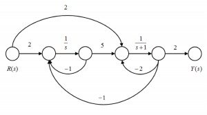
Consider the following signal flow graph, where the system parameters are as follows: [latex]a=1, b=3, c=2, d=1, e=2[/latex].

Apply the Mason’s Gain Formula to find the system transfer function [latex]G(s) = \frac{Y(s)}{R(s)}[/latex]. Once you have the transfer function, find the system poles, zeros, multiplier gain, DC gain, and then write out the transfer function in the TF format as well as in ZPK format. Derive the analytical function describing the step response of this system.

3.3.17 Example

Consider the following signal flow graph representing a certain control system:

Apply the Mason’s Gain Formula to find the system transfer function [latex]G(s) = \frac{Y(s)}{R(s)}[/latex] and write out the transfer function in the TF format (polynomial ratio). Find the analytical expression for a response of the system to a normalized unit step reference.

3.3.18 Example

Consider the following transfer function of a certain process G(s):

[latex]G(s) = \frac{2s+100}{s^{3} + 9s^{2} + 26s + 24}[/latex]

Complete a signal flow graph diagram so that it will represent G(s). Justify your sketch by applying the Mason’s Gain formula to verify the transfer function. Assume that the process G(s) is going to work in a unit feedback closed loop system under Proportional Control. Find the practical range of values for the Controller Gain [latex]K_{p}[/latex] for a stable operation of the closed loop system, and the value of Operational Gain, [latex]K_{op}[/latex] such that the Gain Margin is 2.

3.3.19 Example

Consider the block diagram of a servo-control system for one of the joints of a robot arm, shown next.

The input is the reference angular velocity (speed) for the robot arm, the output is the actual load velocity of the arm, and the forward path contains a Proportional + Integral (PI) Controller, a calibration gain, motor and robotic arm dynamics and a gearbox. The Proportional + Integral (PI) Controller is described as:

[latex]G_{c}(s) = K_{p} + \frac{K_{i}}{s}[/latex]

Find the closed loop system transfer function, [latex]G_{cl}(s)[/latex], in terms of the PI Controller gains, [latex]K_{p}[/latex] and [latex]K_{i}[/latex] Next, find the practical ranges of the controller gains, [latex]K_{p}[/latex] and [latex]K_{i}[/latex], such that the closed loop system is stable.

3.3.20 Example

Consider again the block diagram of the servo-control system for one of the joints of a robot arm, discussed in Example 3.3.19. Apply Mason’s Gain Formula to compute the transfer function of the closed loop system and check to see that the result is the same.

3.3.21 Example

Consider the block diagram of a servo-control system for one of the joints of a robot arm, shown next.

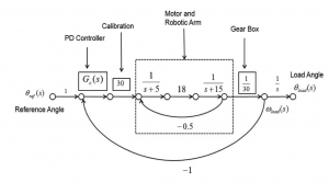
It is very similar to the one in Example 3.3.19, except the input is now the reference angle (position) of the robot arm, and the output is the actual load position of the robotic arm, as opposed to the velocity of the arm. The forward path contains a Proportional + Derivative (PD) Controller, a calibration gain, motor and robotic arm dynamics and a gearbox. Find the closed loop system transfer function, [latex]G_{cl}(s)[/latex], in terms of the PD Controller gains, [latex]K_{p}[/latex] and [latex]K_{d}[/latex]. The Proportional + Derivative (PD) Controller is described as:

[latex]G_{c}(s) = K_{p} + K_{d}s[/latex]

Next, find the practical ranges of the controller gains, [latex]K_{p}[/latex] and [latex]K_{d}[/latex], such that the closed loop system is stable.

3.3.22 Example

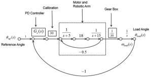
Consider the block diagram of a servo-control system for one of the joints of a robot arm, shown next, very similar to the one in Example 3.3.21, where the input is the reference angle (position) of the robot arm, and the output is the actual load position of the robotic arm. However, observe the small, but significant difference in the placement of the feedback loop. The forward path again contains a Proportional + Derivative (PD) Controller, a calibration gain, motor and robotic arm dynamics and a gearbox. Find the closed loop system transfer function, [latex]G_{cl}(s)[/latex] , in terms of the PD Controller gains, [latex]K_{p}[/latex] and [latex]K_{d}[/latex]. Next, find the practical ranges of the controller gains, [latex]K_{p}[/latex] and [latex]K_{d}[/latex], such that the closed loop system is stable.

3.3.23 Example

Consider a certain process that is represented by the following signal flow graph:

Apply the Mason’s Gain Formula to find the transfer function [latex]G(s)[/latex] it represents. Next, answer the following questions: What is the process DC Gain? What is the process transfer function Gain? What are the initial and final values of the process impulse response? What are the initial and final values of the process step response?

3.3.24 Example

Part 1. Consider a signal flow graph as shown. Find the transfer function [latex]G(s)[/latex] it represents. Show all loop and path gains.

Part 2. The process [latex]G(s)[/latex] is to work in a closed loop configuration as shown next. Find the closed loop transfer function of the system and establish the range of positive gain K values that would result in a stable closed loop system response. Find the critical gain at which the system would be marginally stable.