Chapter 12
12.4 Examples
12.4.1 Example
Recall Example 11.3.2 – we obtained linear approximations of the system process, G(s). Next, assume that the process is to work in a unit feedback closed loop control system, with a Proportional Gain K = 1. Read off your plot created in Example 11.3.2 values of the closed loop system Phase Margin [latex]\Phi_m[/latex] and the corresponding frequency of crossover, [latex]\omega_{cp}[/latex]. Next, use the existing information to create a second order model for the closed loop system.
Based on your model, estimate the transient specifications of the closed loop step response, as well as error specifications of the closed loop responses: [latex]PO,T_{settle},T_{rise},T_{period},K_{pos},e_{ss}(step\%),K_v,e_{ss}(ramp),K_a[/latex] and [latex]e_{ss}(parab)[/latex]. Finally, consider the two traces shown on the plot – which one is the actual closed loop system response, and which one is the model response?
12.4.2 Example
A system is to operate in a unit feedback closed loop configuration and its parameters are not well known, but the closed loop is understood to be stable. Standard frequency response tests are performed on the open loop transfer function, with the controller gain set to 1, as shown:

Obtained open loop frequency response plots are shown below. Find two models for the closed loop system – one based directly on the open loop plots, and one based on the closed loop frequency response (which will have to be computed).
12.4.3 Example
Consider again the unit feedback system under Proportional Control, K, from Example 2.6.12 where the process transfer function G(s) was described as below:
[latex]G(s)=\frac{3000}{(s+1)(s+10)(s+20)}[/latex]
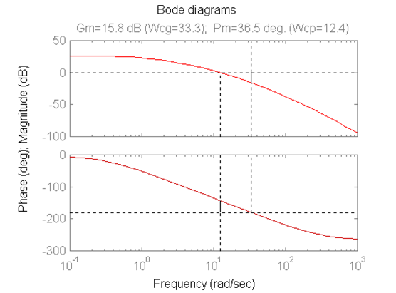
Frequency response plots of the open loop when K = 1 are shown next.
From the open loop process frequency response, [latex]G(j\omega)[/latex], determine the system Gain Margin Gm and Phase Margin, [latex]\Phi_m[/latex], and the corresponding crossover frequencies. Is the closed loop system stable? What is the critical gain, [latex]K_{crit}[/latex], at which the system will be marginally stable? What is the frequency of oscillations, [latex]\omega_{osc}[/latex] , at that gain? Compare your findings with Routh-Hurwitz Criterion results from Example 2.6.12. Next, based on the open loop information, determine the approximate closed loop model of the system, [latex]G_{cl}(s)[/latex], and its parameters, [latex]K_{dc},\zeta,\omega_n[/latex], when proportional Gain K = 1.
12.4.4 Example
A system is to operate in a unit feedback closed loop configuration, and its parameters are not well known, but the closed loop is understood to be stable. Standard frequency response tests are performed on the open loop transfer function, with the controller gain set to 1. Obtained open loop frequency response plots are shown next. Find an appropriate closed loop model for the system.

12.4.5 Example
Consider again the closed loop system from Example 11.3.12. Assuming Controller Gain [latex]K_{op}[/latex] = 1, use the information contained in the frequency response plots to derive two second order approximate models for the closed loop system.
12.4.6 Example
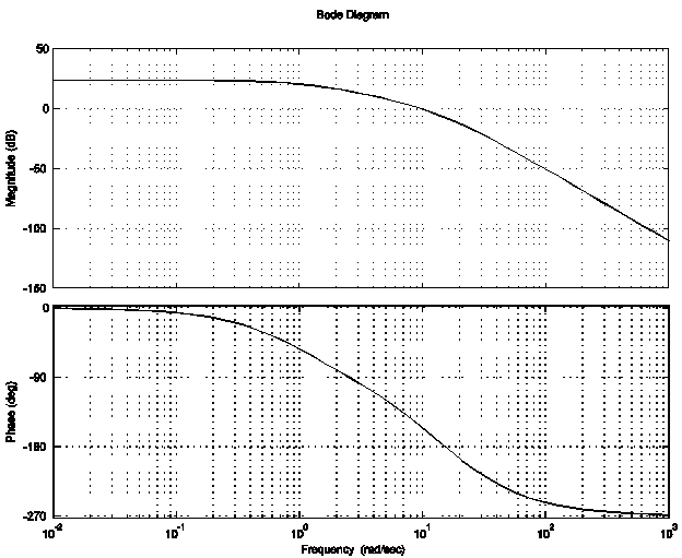
Consider the unit feedback closed loop system under Proportional Control, where the process transfer function G(s) is known:
[latex]G_{open}(s)=\frac{100}{s^3+12.5s^2+26s+10}[/latex]
Frequency response plots of the open and closed loop (assuming Controller Gain = 1) are shown below. Use the information contained in the frequency response plots to derive two second order approximate models for the closed loop system.


12.4.7 Example
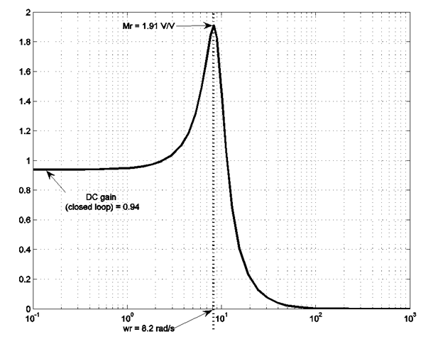
Consider the unit feedback closed loop system under Proportional Control where the process transfer function G(s) is given as:
[latex]G(s)=\frac{750,000}{(s+100)(s+50)(s+5)(s+3)}[/latex]
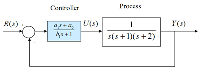
Frequency response plots of the closed loop (note magnitude is in V/V) and the open loop (note magnitude is in dB), both with the Controller Gain [latex]K_{op}[/latex], are shown next. Use the information at hand to derive as many second order approximate models for the closed loop system as you can think of. Next, use these models to obtain estimates of the closed loop system step response, errors and error constants.

12.4.8 Example
Consider again the following closed loop system from Example 11.3.11. Create a second order model for the closed loop system and estimate the specifications of the CLOSED loop properties of the system (system step response, error constants and errors).
12.4.9 Example
Consider again the system from Example 11.3.6. Consider the Root Locus Plot first to decide if a second order model applies to the closed loop system. If the answer is yes, create an appropriate second order and estimate the specifications of the CLOSED loop properties of the system (system step response, error constants and errors).
12.4.10 Example
Consider the following closed loop system compensated by a LEAD Controller. The compensated and uncompensated frequency response plots are shown next.
[latex]G_c(s)=\frac{6s+5}{0.003s+1}[/latex]

The controller was designed to meet the following specifications: a) Closed loop steady state error to a RAMP is to be 0.4 V/V, b) Closed loop step response is to have PO < 20% and [latex]T_{settle}(\pm 2\%)[/latex] < 5 seconds. Predict what the uncompensated step and ramp response would look like. Investigate the feasibility of using a Proportional Controller. Predict what the compensated step and ramp response would look like.
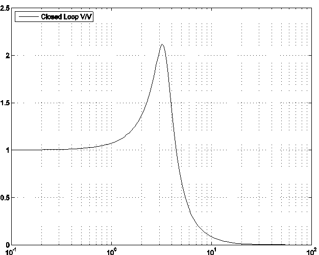
12.4.11 Example
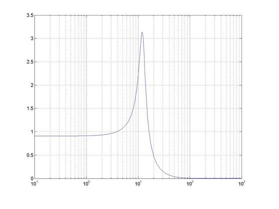
Consider again the unit feedback system under Proportional Control, from the previous example. The Proportional Gain was set to K = 5. Frequency response for the closed loop system was measured experimentally, and its magnitude plot is shown. Note the magnitude is in V/V units. Based on the closed loop data contained in the plot determine the approximate closed loop model of the system, [latex]G_m(s)[/latex], and its parameters [latex]k_{dc},\zeta,\omega_n[/latex].
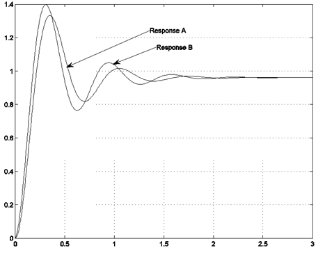
Next, consider now two responses shown in the figure below. One of them corresponds to the actual closed loop system response, and the other to the model response, as it should have been derived in the item above. Identify which one is which and briefly explain why.
12.4.12 Example
Consider a unit feedback system under Proportional Control. OPEN LOOP frequency response plots of KG(s) when K = 1 is shown. When K = 1, determine the approximate CLOSED LOOP model of the system, [latex]G_{m1}(s)[/latex], and its parameters: [latex]k_{dc},\zeta,\omega_n[/latex] Next, consider that the actual closed loop system (with K = 1) has the following poles: -1+j8.85, -1-j8.85 and -18.85. Based on the dominant pair of the closed loop poles, determine another approximate CLOSED LOOP model of the system, [latex]G_{m2}(s)[/latex], and its respective parameters [latex]k_{dc},\zeta,\omega_n[/latex]. Compare the two models – are they similar? Which of the two models will be more accurate? Briefly explain why. Pick the model which you consider the more accurate and based on it, estimate transient specifications of the closed loop step response, as well as error specifications of the closed loop responses: [latex]PO, T_{rise}(10\%-90\%),T_{settle}(\pm 2\%),T_{period}[/latex] and the errors and error constants: [latex]k_{pos},e_{ss}(step\%),K_v,e_ss(ramp),k_a,e_{ss}(parab)[/latex].
12.4.13 Example
Consider again the closed loop control system under Proportional Control from Example 11.3.17. Closed loop frequency response plots of the system with [latex]K_p=1[/latex] are shown next. The closed loop transfer function of the system, when [latex]K_p=1[/latex] has three poles: [latex]p_1=-0.7791+j3.3524[/latex], [latex]p_2=-0.7791+-j3.3524[/latex], [latex]p_3=-8.4418[/latex]. Determine if the second order dominant poles model applies to the closed loop transfer function [latex]G_{m1}(s)[/latex]and if so, derive its transfer function, [latex]G_{m2}(s)[/latex] in the standard form. Refer back to the open loop Bode plots in Example 11.3.17 and determine the second order dominant poles model, [latex]G_{m3}(s)[/latex]from the information provided in the plots. Determine the second order dominant poles model, from the information provided in the closed loop Bode plot above. How do the three models compare? Use the one you consider the most accurate to estimate the following closed loop step response specifications: [latex]e_{ss}(step\%),T_{rise(0-100\%)}[/latex] and PO.