Chapter 12
12.3 Summary
The Phase Margin, [latex]\Phi_m[/latex], is related to the equivalent closed loop damping ratio [latex]\zeta[/latex], which in turn determines the Percent Overshoot of the step response. The relationship is almost linear, as shown in Figure 12‑9, and can be approximated with a very simple linear proportionality in Equation 12‑19 and Equation 12‑20, valid for [latex]0<\zeta<0.65[/latex]:
The graph in Figure 12‑9 can be used to read off the Phase Margin – Damping Ratio values more accurately. Once the damping ratio is estimated, Percent Overshoot of the closed loop step response can be estimated.
The crossover frequency [latex]\omega_{cp}[/latex] relates to the frequency and therefore to the closed loop step response settling time. The equations are based on a 2nd order model for the closed loop system. Note that:
| [latex]\Phi_m=90^0-tan^{-1}\left ( \frac{\omega_{cp}}{2\zeta\omega_{n}} \right )[/latex] [latex]tan(90^0-\alpha)=\frac{1}{tan\alpha}[/latex] [latex]tan(\Phi_m)=\frac{1}{tan(tan^{-1}\left ( \frac{\omega_{cp}}{2\zeta\omega_n} \right ))}=\frac{2\zeta\omega_n}{\omega_{cp}}[/latex] [latex]tan(\Phi_m)=\frac{2\zeta\omega_n}{\omega_{cp}}[/latex] [latex]\omega_n=\frac{tan(\Phi_m)\omega_{cp}}{2\zeta}[/latex] |
Equation 12‑21 |
We can redefine settling time directly from Phase Margin and crossover frequency:
| [latex]T_{settle}(\pm 2 \%)=\frac{4}{\zeta\omega_n}[/latex] [latex]T_{settle}(\pm 2 \%)=\frac{8}{\omega_{cp}tan(\Phi_m)}[/latex] |
Equation 12‑22 |
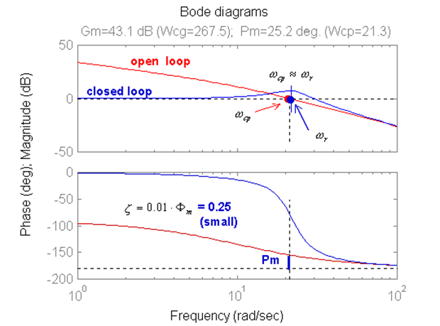
Note that the crossover frequency for Phase Margin is approximately equal to the resonant frequency for the closed loop transfer function if damping ratio is small:
| [latex]\omega_{cp}=\omega_{n}\sqrt{-2\zeta^2+\sqrt{4\zeta^4+1}}\approx \omega_r=\omega_n\sqrt{-2\zeta^2+1}[/latex] | Equation 12‑23 |
Using this relationship gives us an alternative to finding the frequency of natural oscillations [latex]\omega_{n}[/latex]. Rather than computing the closed loop frequency response, which may be tedious, and then reading off the resonant frequency [latex]\omega_{r}[/latex], we can estimate [latex]\omega_{r}[/latex] based on the open loop frequency plot and the value of the crossover frequency, as shown in Equation 12‑23.
These observations are useful in moving back and forth between open loop frequency response, closed loop frequency response and closed loop time (step) response. We will also assume that the higher order systems are approximated well by a 2nd order model (dominant pair of complex poles will be assumed to exist in the closed loop transfer function). Therefore, all relationships derived for the 2nd order model here will be also applicable for the higher order systems. Figure 12‑10 shows the relationship between open loop and closed loop frequency responses.
See the plot in Figure 12‑10 for illustration.


