
Chapter 11
11.1 Gain Margin from Bode Plot
At the critical gain value [latex]K=K_{crit}[/latex] , the system is marginally stable with some roots on the imaginary axis (recall Routh Array):
| [latex]K=K_{crit}[/latex] [latex]s=j\omega _{osc}[/latex] [latex]G(s)H(s)=G(j\omega _{osc})H(j\omega _{osc})[/latex] |
Equation 11‑1 |
The closed loop characteristic equation at [latex]K=K_{crit}[/latex] is:
| [latex]1+KG(s)H(s)=0[/latex] [latex]1+K_{crit}G(j\omega_{osc})H(j\omega_{osc})=0[/latex] [latex]K_{crit}G(j\omega_{osc})H(j\omega_{osc})=-1[/latex] [latex]K_{crit}G(j\omega_{osc})H(j\omega_{osc})=1\angle -180^{0}[/latex] [latex]K_{crit}=\frac{1}{\left | G(j\omega_{osc})H(j\omega_{osc}) \right |}[/latex] [latex]\left | G(j\omega_{osc})H(j\omega_{osc}) \right |=\frac{1}{K_{crit}}[/latex] [latex]\angle G(j\omega_{osc})H(j\omega_{osc})=-180^{0}[/latex] |
Equation 11‑2 |
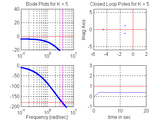
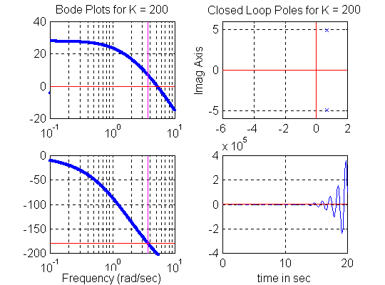
The frequency of oscillations at [latex]K=K_{crit}[/latex] can be established from the phase plot as the frequency at which the phase plot crosses over the [latex]-180^{0}[/latex] line. Then, [latex]K_{crit}[/latex] can be found from the gain plot. Figure 11‑1, Figure 11‑2 and Figure 11‑3 show open loop frequency response plots of a certain system as K changes, with the corresponding closed loop pole locations and the corresponding step response. Watch for the frequency of oscillations at [latex]K=K_{crit}[/latex]at which the phase plot crosses over the [latex]-180^{0}[/latex] line. Based on these plots, a graphical alternative can be found to calculating the Gain margin from the gain and phase equation. Note that since it is customary to use decibel units on frequency response plots, Gain margin will now be also expressed in decibel units, rather than in Volt/Volt units. Recall that:
[latex]G_{m}=\frac{K_{crit}}{K_{op}}[/latex]
- [latex]G_{m}=1[/latex] corresponds to a marginally stable system
- [latex]G_{m}> 1[/latex] corresponds a stable system
- [latex]G_{m}< 1[/latex] corresponds to an unstable system.
The equivalent values of the gain margin in decibels will be then:
- [latex]G_{m}=0[/latex] dB corresponds to the marginally stable system
- [latex]G_{m}> 0[/latex] dB corresponds to the stable system
- [latex]G_{m}< 0[/latex] dB corresponds to the unstable system
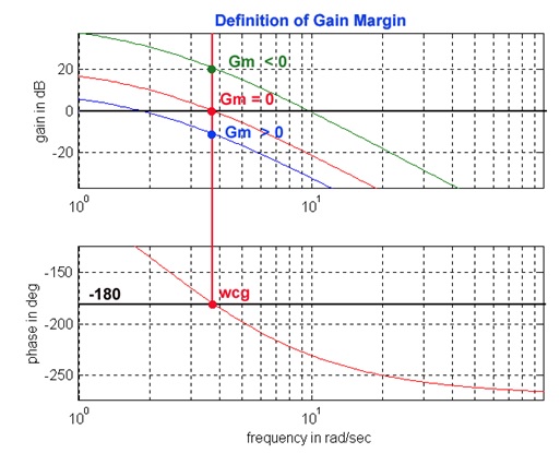
Let the crossover frequency be defined as [latex]\omega_{cg}[/latex] , the frequency at which the phase plot crosses over the [latex]-180^{0}[/latex] line, then let the Gain Margin be defined in dB units:
| [latex]G_{m}=\frac{K_{crit}}{K_{op}}[/latex] [latex]G_{m(dB)}=K_{crit(dB)}-K_{op(dB)}[/latex] |
Equation 11‑3 |

As shown in Figure 11‑4, if the open loop plot [latex]G(j\omega )[/latex] is below the 0 dB axis at the frequency of crossover, [latex]\omega_{cg}[/latex] , then the system has a positive decibel Gain Margin and is stable. If the open loop plot [latex]G(j\omega )[/latex] is above the 0 dB axis at the frequency of crossover, [latex]\omega_{cg}[/latex], then the system has a negative decibel Gain Margin and is unstable. If the open loop plot [latex]G(j\omega )[/latex]crosses the 0 dB axis exactly at the frequency of crossover, [latex]\omega_{cg}[/latex], then the system has a zero decibel Gain Margin and is marginally stable.
Note that [latex]K_{crit}[/latex] and [latex]\omega_{cg}[/latex] can be calculated analytically from the Routh-Hurwitz Criterion. The advantage of using the Gain Margin in frequency domain is that when the system transfer function G(s) is of a higher order, Routh Array calculations become unwieldy. However, Gain Margin in frequency domain can be easily obtained graphically (either from simulations of the open loop frequency response plots or by sketching straight lines approximations – Bode plots).
Moreover, in cases when open loop frequency response plots are obtained experimentally, and the system model is not identified, Gain Margin criterion of stability can still be applied. This allows for a system analysis (and also controller design), without the need to determine an accurate system model, which may be quite an involved procedure. Finally, if a lower order system model is obtained using dominant characteristics, Gain Margin will still accurately reflect higher order system dynamics, which affect the system stability.
