
Chapter 13
13.2 Lead Controller
A transfer function of the lead compensator is a first order combination of a real pole block and a real zero block, with an adjustable gain:
| [latex]G_{c}(s)=K_{c}\cdot\frac{\tau s +1}{\alpha\tau s +1} = \frac{\alpha_1 s + \alpha_0}{b_1 s + 1}[/latex] | Equation 13‑1 |

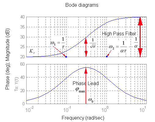
[latex]a_0 = K_c[/latex] corresponds to the DC gain of the controller, and [latex]\alpha < 1[/latex] (the zero is closer to Im axis than the pole). Zero is at: [latex]s_1 = - \frac{a_0}{a_1} = - \frac{1}{\tau}[/latex] Pole is at: [latex]s_2 = - \frac{1}{b_1} = - \frac{1}{\alpha\tau}[/latex] In the frequency domain, the two corner frequencies are: [latex]\omega_1 = \frac{1}{\tau}[/latex] , [latex]\omega_2 = \frac{1}{\alpha\tau}[/latex] The magnitude is described as:
| [latex]M(\omega)=K_c \cdot \frac{\sqrt{{(\omega\tau)}^2 + 1}}{\sqrt{{(\omega\alpha\tau)}^2 + 1}}[/latex] | Equation 13‑2 |
The phase is described by Equation 13‑2 and [latex]\varphi_{max}[/latex] can be calculated from [latex]\frac{d\varpi}{d\omega}=0[/latex]. Resulting in Equation 13-4.
| [latex]\varphi (\omega) = \tan^{-1}\omega\tau - \tan^{-1}\omega\alpha\tau[/latex] | Equation 13‑3 |
| [latex]\varphi_{max} = \sin^{-1}(\frac{1-\alpha}{1+\alpha})[/latex] | Equation 13‑4 |
Magnitude and phase plots are shown in Figure 13-2.
The maximum of phase lead [latex]\varphi_{max}[/latex] occurs at the midpoint frequency as shown in Equation 13‑5:
| [latex]\omega_0 = \sqrt{\omega_1 \omega_2} = \frac{1}{\sqrt{\alpha}\cdot \tau}[/latex] | Equation 13‑5 |
At this frequency the compensator gain is:
| [latex]M(\omega_0) = K_c \frac{\sqrt{{(\omega_0\tau)^2} + 1}}{\sqrt{{(\omega_0\alpha\tau)^2} + 1}} = K_c \frac{\sqrt{{(\frac{1}{\sqrt{\alpha} \tau}\cdot\tau)^2} + 1}}{\sqrt{{(\frac{1}{\sqrt{\alpha} \tau}\cdot\alpha\tau)^2} + 1}} = K_c \frac{\sqrt{{(\frac{1}{\sqrt{\alpha}})^2} + 1}}{\sqrt{{(\frac{1}{\sqrt{\alpha} }\cdot\alpha)^2} + 1}} = K_c \frac{\sqrt{\frac{1}{\alpha} + 1}}{\sqrt{\alpha +1}} = K_c\frac{\sqrt{\frac{1+\alpha}{\alpha}}}{\sqrt{\alpha +1}}[/latex] | |
| [latex]M(\omega_0) = K_c \frac{1}{\sqrt{\alpha}}[/latex] | Equation 13‑6 |
At the high frequency [latex]\omega \rightarrow \infty[/latex], in practical terms, when [latex]\omega >> \frac{1}{\alpha\tau}[/latex] the compensator gain is:
| [latex]M(\omega) = K_c \frac{\sqrt{{(\omega\tau)^2} + 1}}{\sqrt{{(\omega\alpha\tau)^2} + 1}}[/latex] | |
| [latex]\omega \rightarrow \infty[/latex] | |
| [latex]M(\omega) \approx K_c \frac{\sqrt{{(\omega\tau)^2}}}{\sqrt{{(\omega\alpha\tau)^2}}} = K_c[/latex] | |
| [latex]M(\infty)=K_c\cdot \frac{1}{\alpha}[/latex] | Equation 13‑7 |
How to use the Lead Controller:
- Use the phase lead available from the lead parameter [latex]\Phi_m[/latex] to correct deficiencies in the Phase Margin
- Try to increase BOTH [latex]\omega_{cp}[/latex] and [latex]K_{DC(open)}[/latex]
- Adjust as required
13.2.1 Simplified Lead Controller Design
For the simplified design, this form of the Lead Compensator is more convenient:
| [latex]G_c(s) = K_c \cdot \frac{\tau s +1}{\alpha \tau s +1}[/latex] | Equation 13‑8 |
Zero is at [latex]s_1 = - \frac{1}{\tau}[/latex], pole is at [latex]s_2 = - \frac{1}{\alpha\tau}[/latex]. The design will involve first making a decision on what the compensated system phase margin [latex]\Phi_m[/latex] should be and at what frequency [latex]\omega_{cp}[/latex] it should occur. Recall that the phase margin is related to the equivalent closed loop damping ratio [latex]\zeta[/latex], which in turn determines the percent overshoot of the step response:
[latex]\zeta = 0.01\cdot \Phi_m[/latex]
[latex]PO = 100\cdot({e^{\frac{-\zeta\pi}{\sqrt{1-\zeta^2}}}})[/latex]
Dynamic tracking requirements (PO spec) will then be translated into the required [latex]\Phi_m[/latex]. Also, recall that the crossover frequency [latex]\omega_{cp}[/latex] relates to the closed loop model frequency which in turn affects the closed loop step response settling time:
[latex]T_{settle(\pm5\%)}=\frac{3}{\zeta\omega_n}[/latex]
[latex]T_{settle(\pm2\%)}=\frac{4}{\zeta\omega_n}[/latex]
Lead Compensator adds phase lead at the mid-point frequency [latex]\omega_{0}[/latex] as seen in Figure 13‑2. Dynamic tracking requirements (Settling Time spec) will then be translated into the required [latex]\omega_{cp}[/latex]. Once [latex]\omega_{cp}[/latex] is decided, we will assume the maximum phase lift will be placed at this frequency to maximize the Phase Margin:
| [latex]\omega_{cp} = \omega_0[/latex] | Equation 13‑9 |
Once [latex]\Phi_{m} = \omega_0[/latex] is decided, calculate the compensator parameter from the maximum of the phase lead needed:
| [latex]\varphi_{max}=\sin^{-1}({\frac{1-\alpha}{1+\alpha}})[/latex] | Equation 13‑10 |
The compensator time constant [latex]\tau[/latex] can now be calculated:
| [latex]\omega_{cp} = \omega_{0} = \frac{1}{\sqrt{\alpha}\cdot\tau}[/latex] | Equation 13‑11 |
Remember that the additional magnitude added by the lead component at the mid-point frequency is equal to [latex]M(\omega_0)=K_c\frac{1}{\sqrt{\alpha}}[/latex], as shown in Figure 13‑2. This will shift the crossover frequency [latex]\omega_{cp}[/latex] from its intended position at [latex]\omega_{0}[/latex], and will affect the Phase Margin. To re-adjust the crossover frequency, change the DC gain of the controller, [latex]K_{c}[/latex]. Note that the resulting open loop gain may or may not meet the error specification.
NOTE:
This design is simple but does not allow meeting the closed loop steady state error specification directly. When the system is Type 1 and the step error is of no concern, this approach works best. Notice that since the DC gain of the controller is adjusted last, to achieve at the same time an improvement in the system tracking as well may require many trial-and-error iterations. This may prove tedious, or impossible, and so this simple approach should be mainly used if improving the tracking accuracy is not important, for example, when the system already has high error constants and therefore a good steady state tracking. This approach allows meeting the design requirements w.r.t. damping (percent overshoot) and speed (settling time) with relatively few calculations.
13.2.2 Analytical Lead Controller Design
When achieving the DC tracking accuracy is as important as the dynamic tracking, a different, more analytical approach is recommended, which will allow you to find a lead network with a specific DC gain, that will create a specified Phase Margin [latex]\Phi_{m}[/latex] at a specified crossover frequency, [latex]\omega_{cp}[/latex] . Recall that the transfer function of the lead compensator is:
[latex]G_c(s)=\frac{a_1s+a_0}{b_1+1}[/latex]
Coefficient [latex]a_{0}[/latex] corresponds to the DC gain of the controller. Zero is at [latex]s_1 = -\frac{a_0}{a_1}[/latex], pole is at [latex]s_2 = -\frac{1}{b_1}[/latex], as shown in Figure 13‑1. Dynamic tracking requirements dictate what values of the Phase Margin [latex]\Phi_m[/latex] and of the crossover frequency [latex]\omega_{cp}[/latex] should be chosen. Ideally, we want to have the specified Phase Margin [latex]\Phi_m[/latex] to occur at the specified frequency [latex]\omega_{cp}[/latex]. Note that the new crossover frequency [latex]\omega_{cp}[/latex] should be chosen to be larger than the uncompensated one. The condition is written as:
| [latex]G_c(j\omega_{cp})GH(j\omega_{cp}) = 1\angle (-180^\circ + \Phi_m)[/latex] | |
| [latex]\frac{a_1j\omega_{cp} + a_0}{b_1j\omega_{cp}+1}GH(j\omega_{cp}) = 1\angle (-180^\circ + \Phi_m)[/latex] | Equation 13‑12 |
The above complex equation results in two conditions (magnitude and phase), with two unknowns, [latex]a_{1}[/latex] and [latex]b_{1}[/latex]:
| [latex]\left | \frac{a_1j\omega_{cp} + a_0}{b_1j\omega_{cp}+1}GH(j\omega_{cp}) \right | = 1[/latex] | |
| [latex]\tan^{-1}(\frac{a_1j\omega_{cp}}{a_0})-\tan^{-1}(b_1j\omega_{cp}) = -180^{\circ}+\Phi_m[/latex] | Equation 13‑13 |
The two equations can be then solved. It is convenient to define the following “Phase Lift” angle [latex]\theta[/latex]:
| [latex]\theta = -180^{\circ} + \Phi_m - \angle G(j\omega_{cp})[/latex] | Equation 13‑14 |
The Lead Controller coefficients are then calculated as:
| [latex]a_1 = \frac{1 - a_0\cdot\left | G(j\omega_{cp}) \right |\cdot\cos{\theta}}{\omega_{cp}\cdot\left | G(j\omega_{cp}) \right |\cdot\sin{\theta}}[/latex] | |
| [latex]b_1 = \frac{\cos{\theta} - a_0 \cdot \left | G(j\omega_{cp}) \right |}{\omega_{cp}\cdot\sin{\theta}}[/latex] | Equation 13‑15 |
Observation I:
Note that although the solution to these equations will always exist, not all solutions will be acceptable. If [latex]a_{1}[/latex] is negative, the Lead Controller will be non-minimum phase. If [latex]b_{1}[/latex] is negative, the Lead Controller is unstable. If either of these cases occurs, the initial choices of [latex]\Phi_{m}[/latex], [latex]\omega_{cp}[/latex] have to be modified until positive solutions are found.
Observation II:
Note that if [latex]\omega_{cp}[/latex] for the compensated system is chosen to be less than that of the uncompensated system, we will end up with a Lag Controller transfer function, shown in Equation 13‑16, where [latex]a_0 = K_c[/latex] corresponds to the DC gain of the controller, and [latex]a<1[/latex] (i.e. the controller pole is closer to Im axis than the zero).
