
Chapter 7
7.2 Response Specifications for the Second Order Underdamped System
7.2.1 Percent Overshoot
Peak Time is defined as the time the oscillatory response reaches its maximum, as shown in Figure 7‑3. let us assume that the process is described by the transfer function in Equation 7‑1. The Peak Time can be found as the time corresponding to the maximum of the system step response. The maximum of a function is found by taking the derivative and setting it to zero, but rather than finding the maximum of the time function, we use the Laplace Transform domain, as shown in Equation 7‑6.
| [latex]y_{step}(s) \Rightarrow \frac{1}{s}\cdot K_{dc} \cdot\frac{\omega^{2}_{n}}{s^{2}+2\zeta\omega_{n}s + \omega_{n}^{2}}[/latex] | |
| [latex]\frac{dy_{step}(t)}{dt} \Rightarrow sY(s)= s \cdot\frac{1}{s}\cdot K_{dc} \cdot\frac{\omega^{2}_{n}}{s^{2}+2\zeta\omega_{n}s + \omega_{n}^{2}} = K_{dc}\cdot \frac{\omega^{2}_{n}}{s^{2}+2\zeta\omega_{n}s + \omega_{n}^{2}}[/latex] | |
| [latex]\frac{dy_{step}(t)}{dt} = 0 \Rightarrow \frac{dy_{step}(t)}{dt}[/latex] | |
| [latex]= L^{-1} \Bigg \{K_{dc}\cdot \frac{\omega^{2}_{n}}{s^{2}+2\zeta\omega_{n}s + \omega_{n}^{2}} \Bigg \} \Rightarrow L^{-1} \Bigg \{K_{dc}\cdot \frac{\omega^{2}_{n}}{s^{2}+2\zeta\omega_{n}s + \omega_{n}^{2}} \Bigg \} = 0[/latex] | |
| [latex]\frac{dy_{step}(t)}{dt} = L^{-1} \Bigg \{K_{dc}\cdot \frac{\omega^{2}_{n}}{s^{2}+2\zeta\omega_{n}s + \omega_{n}^{2}} \Bigg \}[/latex] | |
| [latex]= K_{dc} \cdot \frac{\omega_{n}e^{-\zeta\omega_{n}t}}{\sqrt{1-\zeta^{2}}}sin\bigg(\omega_{n}\sqrt{1-\zeta^{2}}t\bigg)\cdot 1(t)[/latex] | |
| [latex]\frac{dy_{step}(t)}{dt} = 0 \rightarrow K_{dc} \cdot \frac{\omega_{n}e^{-\zeta\omega_{n}t}}{\sqrt{1-\zeta^{2}}}sin\bigg(\omega_{n}\sqrt{1-\zeta^{2}}t\bigg)\cdot 1(t) = 0[/latex] | |
| [latex]sin(\omega_{n}\sqrt{1-\zeta^{2}}t)\cdot 1(t) = 0 \rightarrow \omega_{n}\sqrt{1-\zeta^{2}}t \rightarrow \omega_{d}t = 0[/latex] | |
| [latex]\omega_{d}T_{peak}=0\pm n\pi=0, \pi, 2\pi ...[/latex] | Equation 7-6 |
The time [latex]T_{peak}[/latex] when y(t) reaches its maximum is at [latex]\omega_{d}T_{peak} = \pi[/latex]
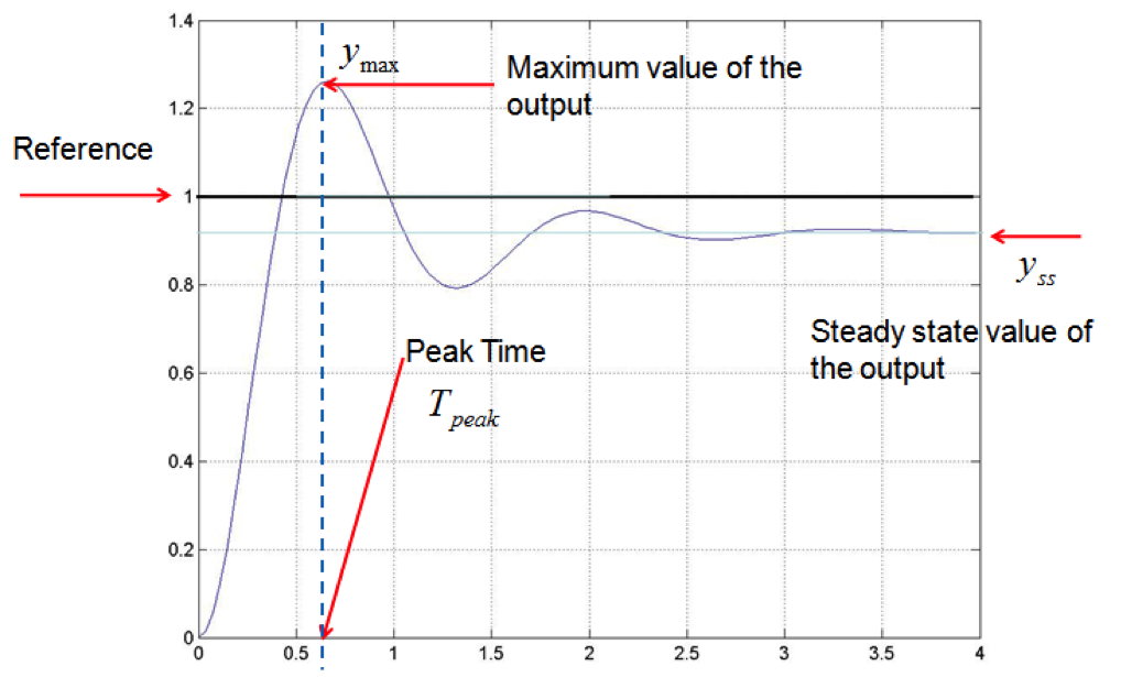
From Equation 7‑6 we now can calculate the Peak Time, [latex]T_{peak}[/latex]:
| [latex]T_{peak} = \frac{\pi}{\omega_{d}} = \frac{\pi}{\omega_{n}\sqrt{1-\zeta^{2}}}[/latex] | Equation 7-7 |
Percent Overshoot can now be found by substituting the Peak Time, [latex]T_{peak}[/latex] into the step response function described by Equation 7‑5:
| [latex]y_{max}(t) = y_{step}(T_{step})=K_{dc}\cdot \Bigg( 1-\frac{e^{-\zeta\omega_{n}T_{peak}}}{\sqrt{1-\zeta^{2}}} sin\bigg(\omega_{d}\frac{\pi}{\omega_{d}}+\phi \bigg) \Bigg)\cdot 1(t)[/latex] | Equation 7-8 |
To solve Equation 7‑8, use the trigonometrical formula for the sine of a sum of two angles:
[latex](sin(\pi + \phi)) = sin(\pi)\cdot cos(\pi) + cos(\pi) \cdot sin(\phi) = 0 - sin(\phi) = -sin(\phi)[/latex]
Recall that from Figure 7‑2 we have:
[latex]sin(\phi) = \sqrt{1-\zeta^{2}}[/latex]
Thus:
[latex](sin(\pi + \phi)) = -sin(\phi) = -\sqrt{1-\zeta^{2}}[/latex]
Substitute this into Equation 7‑8 for the output maximum:
| [latex]y_{max}(t) = y_{step}(T_{step})=K_{dc}\cdot \Bigg( 1-\frac{e^{-\zeta\omega_{n}T_{peak}}}{\sqrt{1-\zeta^{2}}} sin\bigg(\omega_{d}\frac{\pi}{\omega_{d}}+\phi \bigg) \Bigg)\cdot 1(t)[/latex] | |
| [latex]= K_{dc}\cdot \bigg(1 + e^{-\zeta\omega_{n}T_{peak}} \bigg) = K_{dc} \cdot\Bigg( 1+e^{-\zeta\omega_{n}\frac{\pi}{\omega_{n}\sqrt{1-\zeta^{2}}}}\Bigg)[/latex] | Equation 7-9 |
Finally, we can use the defining equation describing the Percent Overshoot, i.e. Equation 4‑2:
| [latex]PO = \frac{y_{max} - y_{ss}}{y_{ss}}\cdot 100\% = \frac{y_{max} - K_{dc}}{y_{ss}}\cdot 100\%[/latex] | |
| [latex]PO = 100 \cdot \Bigg( e^{\frac{-\zeta\pi}{\sqrt{1-\zeta^{2}}}}\Bigg)[/latex] | Equation 7-10 |
The relationship between Percent Overshoot PO and damping ratio [latex]\zeta[/latex] is inversely proportional, as shown in Figure 7‑4: The smaller the damping ratio, the larger the overshoot. When [latex]\zeta = 0[/latex] , the system is marginally stable, i.e. the response show undamped oscillations of a constant amplitude, and PO = 100%.
Equation 7‑10 can be also solved for damping ratio if the Percent Overshoot is known, but it is tedious, hence the suggestion to use Figure 7‑4 to read off the value [latex]\zeta[/latex] rather than compute it. The computation, if performed, would be as follows – start with taking a natural log of both sides of the equation:
| [latex]PO = 100 \cdot \Bigg( e^{\frac{-\zeta\pi}{\sqrt{1-\zeta^{2}}}}\Bigg)[/latex] | |
| [latex]ln\bigg(\frac{PO}{100} \bigg) = \frac{ -\zeta\pi}{\sqrt{1-\zeta^{2}}}[/latex] | |
| [latex]\zeta\pi = -ln\bigg(\frac{PO}{100} \bigg)\sqrt{1-\zeta^{2}}[/latex] [latex]\zeta^{2}\pi^{2} = \bigg(-ln\bigg(\frac{PO}{100} \bigg)\bigg)^{2}(1-\zeta^{2})[/latex] |
|
| [latex]\bigg(\pi^{2} + \bigg(-ln\bigg(\frac{PO}{100} \bigg)\bigg)^{2}\bigg) \cdot \zeta^{2} = \bigg(-ln\bigg(\frac{PO}{100} \bigg)\bigg)^{2}[/latex] | |
| [latex]\zeta = \sqrt{\frac{\bigg(-ln\bigg(\frac{PO}{100} \bigg)\bigg)^{2}}{\bigg(\pi^{2} + \bigg(-ln\bigg(\frac{PO}{100} \bigg)\bigg)^{2}\bigg)}}[/latex] | Equation 7-11 |

7.2.2 Settling Time
Recall the definition of the Settling Time, as shown in Figure 4‑3. Also recall that the exponential decays to approximately 5% of its original value after three Time Constants (i.e. 3[latex]\tau[/latex]) and to approximately 2% of its original value after approximately four Time Constants (i.e. 4[latex]\tau[/latex]). Thus, the function [latex]1-e^{\frac{t}{\tau}}[/latex] will reach approximately 95% of its steady state value (i.e. ), after[latex]t = 3\tau[/latex] , and will reach approximately 98% of its steady state value (i.e. 1), after [latex]t = 4\tau[/latex]:
[latex]e^{-\frac{3\tau}{\tau}} = e^{-3} = 0.0498, 1-e^{-\frac{3\tau}{\tau}} = e^{-3} = 0.9502[/latex]
[latex]e^{-\frac{4\tau}{\tau}} = e^{-4} = 0.0183, 1-e^{-\frac{4\tau}{\tau}} = e^{-4} = 0.9817[/latex]
Now recall that the step response of the second order underdamped system in Equation 7‑5 is an exponentially damped sine function. The Time Constant of the exponential envelope is shown in Equation 7‑12:
| [latex]\tau = \frac{1}{\sigma} = \frac{1}{\zeta\omega_{n}}[/latex] | Equation 7-12 |
Therefore, the two definitions of the Settling Time can be described as follows:
| [latex]T_{settle(\pm 2\%)} = \frac{4}{\zeta\omega_{n}}[/latex] | Equation 7-13 |
| [latex]T_{settle(\pm 5\%)} = \frac{3}{\zeta\omega_{n}}[/latex] | Equation 7-14 |
7.2.3 Rise Time
Recall the definition of the Rise Time, as shown in Figure 4‑4. Consider the 0 to 100% definition – we are looking for the time where the step response output crosses for the first time the steady state value, [latex]y_{ss}[/latex]. The steady state value of the step response as calculated in Equation 7‑5, is equal to the DC gain:
| [latex]y_{ss}=\lim_{t\rightarrow\infty}y_{step}(t)[/latex] | |
| [latex]=\lim_{t\rightarrow\infty}\Bigg \{K_{dc}\cdot \Bigg ( 1-\frac{e^{-\zeta\omega_n t}}{\sqrt{1-\zeta^2}} \sin{(\omega_n\sqrt{1-\zeta^2}t + \cos^{-1}\zeta)} \Bigg)\cdot1(t)\Bigg \} = K_{dc}[/latex] | Equation 7-15 |
Therefore, when [latex]t = T_{rise(0-100\%)}[/latex], we have the output equal to DC gain:
[latex]y(T_{rise(0-100\%)})=y_{ss}=K_{dc}[/latex]
At the same time, substituting [latex]T_{rise(0-100\%)}[/latex]we have:
[latex]y(T_{rise(0-100\%)}) = K_{dc} \cdot \Bigg( 1 - \frac{e^{\zeta\omega_{n}T_{rise(0-100\%)}}}{\sqrt{1-\zeta^{2}}} sin\bigg( \omega_{d}T_{rise(0-100\%)} + \phi \bigg) \Bigg)[/latex]
What follows is:
| [latex]K_{dc} = K_{dc} \cdot \Bigg( 1 - \frac{e^{\zeta\omega_{n}T_{rise(0-100\%)}}}{\sqrt{1-\zeta^{2}}} sin\bigg( \omega_{d}T_{rise(0-100\%)} + \phi \bigg) \Bigg)[/latex] | |
| [latex]\frac{e^{\zeta\omega_{n}T_{rise(0-100\%)}}}{\sqrt{1-\zeta^{2}}} sin\bigg( \omega_{d}T_{rise(0-100\%)} + \phi \bigg) = 0[/latex] | |
| [latex]sin\bigg( \omega_{d}T_{rise(0-100\%)} + \phi \bigg) = 0[/latex] | |
| [latex]T_{rise(0-100\%)} = \frac{\pi - \phi}{\omega_{d}} = \frac{\pi - cos^{-1}\zeta}{\omega_{n}\sqrt{1-\zeta^{2}}}[/latex] | |
| [latex]T_{rise(0-100\%)} = \frac{\pi - cos^{-1}\zeta}{\omega_{n}\sqrt{1-\zeta^{2}}}[/latex] | Equation 7-16 |
Next, we will use a linear approximation to find the Rise Time from 10% of the steady state to 90% of the steady state – we will assume that the 80% increase of the output corresponds to 80% of the time it takes for the output to increase from 0 to 100%:
| [latex]T_{rise(10-90\%)} \approx 0.8 \cdot T_{rise(0-100\%)}[/latex] | |
| [latex]T_{rise(10-90\%)} \approx 0.8 \cdot\frac{\pi - cos^{-1}\zeta}{\omega_{n}\sqrt{1-\zeta^{2}}}[/latex] | Equation 7-17 |
It can be shown empirically (i.e. by observation), that Equation 7‑17 can also be approximated by another very simple relationship:
| [latex]T_{rise(10-90\%)} \approx \frac{1.8}{\omega_{n}}[/latex] | Equation 7-18 |
7.2.4 Steady State Error
Recall the steady state value of the step response, shown in Equation 7‑15 for the normalized unit input ([latex]r_{ss} = 1[/latex]) is equal to: [latex]y_{ss} = K_{dc}[/latex]. Note that, in general, [latex]y_{ss} = K_{dc} \cdot r_{ss}[/latex], where the constant reference could be non-unit. Next, substitute it to the definition of the steady state error in Equation 4‑3:
| [latex]y_{ss} = K_{dc} \cdot r_{ss}[/latex] | |
| [latex]e_{ss} = r_{ss} - y_{ss}[/latex] | |
| [latex]e_{ss\%} = \frac{r_{ss} - y_{ss}}{r_{ss}} \cdot 100\% = \frac{r_{ss}(1-K_{dc})}{r_{ss}} \cdot 100\%[/latex] | |
| [latex]e_{ss\%} = (1-K_{dc})\cdot 100\%[/latex] | Equation 7-19 |
Equation 7‑19 means that to minimize the closed loop steady state error, the closed loop DC gain, [latex]K_{dc}[/latex], should be as close to 1 as possible. We can also look at the closed loop steady state error by considering the open loop DC gain, [latex]K_{dco} = G_{open}(0)[/latex]. Increasing the open loop DC gain, [latex]K_{dco} \rightarrow \infty[/latex], brings the closed loop DC gain closer to 1: [latex](K_{dc} \rightarrow 1)[/latex] , and thus also reducing the closed loop steady state error. The relationship between the open loop DC gain and the closed loop DC gain is:
| [latex]\frac{K_{dco}}{1+K_{dco}}[/latex] | Equation 7-20 |
The relationship between the closed loop steady state error and the open loop DC gain therefore is:
| [latex]e_{ss\%} = 100(1-K_{dc}) = 100 \bigg(1-\frac{K_{dco}}{1+K_{dco}} \bigg)[/latex] | |
| [latex]e{ss\%} = 100 \bigg( \frac{1}{1+K_{dco}} \bigg)[/latex] | Equation 7-21 |
Equation 7‑21 reinforces what we also see in Equation 7‑19 – that to minimize the steady state error, the open loop DC gain has to be as large as possible without destabilizing the system: [latex]K_{dco} \rightarrow \infty[/latex] .
Now recall that the open loop DC gain is also a definition of the Error Position Constant:
[latex]K_{pos} = \lim_{s \rightarrow 0}G_{open}(s) = K_{dco}[/latex]
Therefore, Equation 7‑21 is the same as Equation 5‑7. If the Position Constant, [latex]K_{pos}[/latex], has a constant value, [latex](K_{pos} = const)[/latex], the System Type is equal to and the steady state error always exists. Recall from Chapter 5.2.1, that to reduce the steady state error to zero, [latex]e_{ss}=0[/latex], the Error Position Constant, [latex]K_{pos}[/latex], which is the same as the open loop DC gain, [latex]K_{dco}[/latex], has to be equal to infinity, [latex]K_{pos} = K_{dco} = \infty[/latex], and the System Type becomes equal to 1 (the open loop transfer function has one integrator).
