13.1 Basic Rules – Summary

Frequency Response-based design is based on several simple assumptions. Relationships between system parameters ([latex]K_{dc}, \zeta, \omega_{n}[/latex]), open loop frequency response, closed loop frequency response and closed loop step response are derived assuming that in most simple cases the closed loop system can be modeled reasonably well by a second order model (dominant complex poles) even if the actual system dynamics are of a higher order:

[latex]G_{m}(s)\approx K_{dc} \frac{\omega_{n}^2}{s^2+\zeta \omega_{n}s + \omega_{n}^2}[/latex]

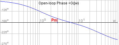
Phase Margin (found on Open Loop Frequency Response Plot) determines PO in Closed Loop Step Response

Phase Margin, [latex]\Phi_{m}[/latex], identified on the open loop frequency response plot, affects the oscillations in the closed loop step response. Recall that the accurate relationship is:

[latex]\Phi_{m} = \tan^{-1} (\frac{2\zeta}{\sqrt{-2\zeta^2 + \sqrt{4\zeta^4+1}}})[/latex]

Use the accurate graph on the left. If the graph is not available, use an approximate relationship [latex]\zeta \approx 0.01 \cdot \Phi_{m}[/latex] for [latex]0 < \Phi_{m} < 15 ^\circ[/latex] and [latex]55^\circ < \Phi_{m}<60^\circ[/latex] or [latex]\zeta\approx 0.01\cdot (\Phi_{m}-4^\circ )[/latex] for [latex]15^\circ < \Phi_{m} < 55^\circ[/latex]

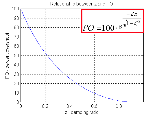
Damping ratio, in turn, decides about the oscillations in the closed loop system step response, i.e. Percent Overshoot:

[latex]PO = 100 \cdot (e^\frac{-\zeta\pi}{\sqrt{1-\zeta^2}} )[/latex]

Small [latex]\Phi_{m}[/latex] corresponds to a small equivalent damping ratio that results in large oscillations (PO):

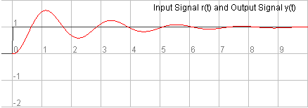
A decent [latex]\Phi_{m}[/latex] (45 – 65 degrees) corresponds to a decent damping ratio (0.4 – 0.7) and small oscillations (small PO):

Frequency of Crossover (found on Open Loop Frequency Response Plot) determines Settling Time in Closed Loop Response

Crossover frequency for Phase Margin, [latex]\omega_{cp}[/latex] (frequency at which the system open loop gain crosses the 0dB line), affects the speed of the closed loop step response:

[latex]\omega_{n} = \frac{\tan (\Phi_m) \cdot\omega_{cp}}{2\zeta}[/latex]

Notice that the Settling Time is inversely proportional to the crossover frequency, [latex]\omega_{cp}[/latex] :

[latex]T_{settle(\pm2\%)} = \frac{4}{\zeta\omega_n}[/latex]     [latex]T_{settle(\pm2\%)} = \frac{8}{\omega_{cp}\cdot\tan(\Phi_m)}[/latex]

Small [latex]\omega_{cp}[/latex] corresponds to slow responses in time domain, and large [latex]\omega_{cp}[/latex] corresponds to fast responses in time domain. Also notice that from the derivation for the Phase Margin, [latex]\omega_{cp}[/latex] is equal to:

[latex]{(\frac{\omega_{cp}}{\omega_{n}})}^2 = -2\zeta^2 + \sqrt{4\zeta^4+1}[/latex]

then:

[latex]\omega_{cp} = \omega_{n}\sqrt{-2\zeta^2 + \sqrt{4\zeta^4+1}}[/latex]

[latex]\omega_{cp} \approx \omega_{n}\sqrt{-2\zeta^2+1}[/latex]

[latex]\omega_{r} = \omega_{n}\sqrt{1 - 2\zeta^2}[/latex]

[latex]\omega_{cp} \approx \omega_{r}[/latex]

This indicates that the crossover frequency \omega_{cp} (found on the open loop plot) and the resonant frequency \omega_{r} (found on the closed loop plot) are practically identical.

Open loop DC Gain determines Steady State Errors in Closed Loop Response

Note that the best (most accurate) way to determine the closed loop step response error is to use an analytical expression for an open loop transfer function, if available, since:

[latex]K_{DC(open)} = K_{pos} =  \lim_{s\rightarrow 0} G_{open}(s)[/latex]

[latex]e_{ss} = \frac{1}{1 + K_{pos}} = \frac{1}{1+K_{DC(open)}}[/latex]

If an expression for the closed loop transfer function is available, we can use the closed loop DC gain as well:

[latex]K_{DC(closed)} = \lim_{s\rightarrow0}G_{closed}(s)[/latex]

[latex]e_{ss}=1-K_{DC(closed)}[/latex]

If only a frequency plot is available, then the DC gain (open or closed loop) can be read off of it, but it will be not as accurate, particularly if the scale is in dB. Any readout in dB will have to be converted to the V/V units before the above formulae can be used.

SUMMARY

The general idea behind the frequency domain-based design is to shape the open loop frequency response so that:

1. [latex]\Phi_{m}[/latex] in 45-65 degrees range is achieved  – so that the equivalent damping ratio [latex]\zeta[/latex] of the closed loop is kept within the 0.4 to 0.7 range, which in turn should result in a PO between 25% (for [latex]\zeta[/latex] = 0.4) and 5% (for [latex]\zeta[/latex] = 0.7).
2. [latex]\omega_{cp}[/latex] is as large as possible – so that the equivalent closed loop frequency of natural oscillations [latex]\omega_{n}[/latex] large, which in turn should result in short Settling and Rise Times;
3. Open Loop DC gain, [latex]K_{dc(open)}[/latex], is as large as possible- so that the closed loop DC gain is as close to 1 as possible, which in turn will minimize the closed loop steady state error.

NOTE: because of the approximate nature of the modelling based on the assumption of a 2nd order dominant poles model, all compensation designs based on it should be verified through simulation, and fine-tuned if necessary.