
Chapter 10
10.7 Evans Root Locus Construction Rule # 5: Crossover with Imaginary Axis
This Rule deals with crossovers with the Imaginary axis and provides an alternative way of finding the critical gain and the frequency of marginal oscillations that can also be found using the Routh-Hurwitz stability criterion.
|
Rule 5: Imaginary axis crossings are found by solving the characteristic equation for the critical value of the gain, [latex]K=K_{crit}[/latex] . Since the equation is complex, it yields two conditions (for Im and Re parts) and thus both the critical gain and the frequency of oscillations can be computed.
|
In our example, the crossovers with Imaginary axis are:
[latex]1+KG(s)=0[/latex]
[latex]s^3+17s^2+80s+100+10K=0[/latex]
[latex]K=K_{crit}[/latex] [latex]s=j\omega_{osc}[/latex]
[latex](j\omega_{osc})^3+[/latex] [latex]17(j\omega_{osc})^2+[/latex] [latex]80(j\omega_{osc})+[/latex] [latex]100+10K_{crit}=0[/latex]
[latex]-j\omega_{osc}^3[/latex] [latex]-17\omega_{osc}^2[/latex] [latex]+j80\omega_{osc}[/latex] [latex]+100+[/latex] [latex]10K_{crit}=0[/latex]
[latex]Re[/latex] [latex]\{-j\omega_{osc}^3[/latex] [latex]-17\omega_{osc}^2+[/latex] [latex]j80\omega_{osc}+[/latex] [latex]100+[/latex] [latex]10K_{crit}\}=0[/latex]
[latex]-17\omega_{osc}^2+[/latex] [latex]100+[/latex] [latex]10K_{crit}=0[/latex]
[latex]Im[/latex] [latex]\{-j\omega_{osc}^3[/latex] [latex]-17\omega_{osc}^2+[/latex] [latex]j80\omega_{osc}+[/latex] [latex]100+[/latex] [latex]10K_{crit}\}=0[/latex]
[latex]-\omega_{osc}^3+80\omega_{osc}=0[/latex]
[latex](-\omega_{osc}^2+80)\omega_{osc}=0[/latex]
[latex]\omega_{osc}^2=80[/latex]
[latex]\omega_{osc}=\sqrt{80}=8.94[/latex]
[latex]-17\cdot80+100+10K_{crit}=0[/latex]
[latex]K_{crit}=\frac{1360-100}{10}=126[/latex]
The final answer is [latex]\omega_{osc}=8.94[/latex] rad/sec and [latex]K_{crit}=126[/latex]

We can verify this using the Routh-Hurwitz Criterion. The system Closed Loop Transfer Function is:
[latex]G_{cl}(s)=\frac{G(s)}{1+G(s)}=[/latex] [latex]\frac{\frac{10K}{s^3+17s^2+80s+100}}{1+\frac{10K}{s^3+17s^2+80s+100}}[/latex]
[latex]G_{cl}(s)=\frac{10K}{s^3+17s^2+80s+(100+10K)}[/latex]
Apply the Routh-Hurwitz criterion to the closed loop characteristic equation:
[latex]s^3+17s^2+80s+(100+10K)=0[/latex]
The necessary condition is:
[latex]100+10K >0[/latex]
K>-10
Sufficient conditions from Routh Array:
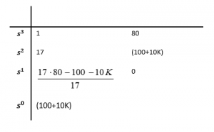
The resulting condition is:
[latex]17 \cdot 80-100-10K>0[/latex]
[latex]K<126[/latex]
What happens when the gain reaches the critical value? When [latex]K=126[/latex]:
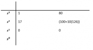
[latex]Q_{aux}(s)=17s^2+1360[/latex] [latex]s^2+80=0[/latex]
[latex]Q_{aux}(s)=0[/latex] [latex]s_1=j \sqrt{80}=j8.94[/latex]
[latex]s_2=-j \sqrt{80}=-j8.94[/latex]
Thus, when [latex]K_{crit}=126[/latex], from the Auxilliary Equation we have: [latex]\omega_{osc}=8.94[/latex] rad/sec. We can also verify this result by using the MATLAB subroutine “rlocfind“.
