
Chapter 10
10.9 Examples
10.9.1 Example
Consider a unit feedback closed loop system under Proportional Control where the open loop process [latex]G(s)[/latex] is given by the equation below, and sketch a Root Locus plot for this system.
[latex]G(s)=\frac{1}{(s+1)(s+3)(s+5)}[/latex]
10.9.2 Example
Consider a unit feedback system with a process described below. Sketch the Root Locus for the system.
[latex]G(s)=\frac{s+0.5)(s+1)}{(s+3)(s+4)}[/latex]
10.9.3 Example
Consider a certain closed loop unit feedback control system under Proportional Control (Gain ) where the process transfer function is as follows:
[latex]G(s) = \frac{(s+2)}{s(s+1)(s+3)(s+5)}[/latex]
See the Root Locus plot for this system, shown below. Determine the critical value of the gain, [latex]K_{crit}[/latex] at which the system becomes marginally stable, and the corresponding frequency of marginally stable oscillations, [latex]\omega_{osc}[/latex].
Apply the Routh-Hurwitz Criterion of Stability to determine the critical value of the gain, [latex]K_{crit}[/latex], at which the system becomes marginally stable, and the corresponding frequency of marginally stable oscillations, [latex]\omega_{osc}[/latex]. Determine the range of gains [latex]K_p[/latex] to provide a stable closed loop system response. How do they compare to item 1)?
10.9.4 Example
Consider a unit feedback system with a process as described.
[latex]G_{open}(s)=K \cdot G(s)[/latex] [latex]=K \cdot \frac{1}{s(s+2)(s+3)}[/latex]
Where [latex]K[/latex] is an adjustable proportional gain controller and [latex]G(s)[/latex] is a process transfer function. Sketch a Root Locus of the closed loop system poles for [latex]0<[/latex] [latex]K[/latex]< [latex]+ \infty[/latex] in the space provided in Figure below. Calculate values of the centroid [latex]\sigma[/latex], asymptotes [latex]\theta[/latex], breakaway points, if any, as well as coordinates of the crossovers with the imaginary axis, if any.
An equivalent damping ratio,[latex]\zeta[/latex] , of the closed loop step response, equal to 0.707, is required. From the root locus plot, find the corresponding value of the controller gain [latex]K[/latex]. Calculate the closed loop system transfer function, [latex]G_{cl}[/latex], for this value of [latex]K[/latex] . Suppose that we increase [latex]K[/latex] up from the value found in [latex]2[/latex]. Complete the following table:
| Percent Overshoot will | Increase | Decrease | Insufficient information to make a decision |
| Settling Time will | Increase | Decrease |
Insufficient information to make a decision |
| Rise Time will | Increase | Decrease | Insufficient information to make a decision |
| Steady State Error to a Ramp Input will | Increase | Decrease | Insufficient information to make a decision |
10.9.5 Example
Consider a unit feedback system with a process as follows, working under Proportional Control:
[latex]G(s)= \frac{1}{s(s+2)(s+3)(s+5)}[/latex]
Apply the Routh-Hurwitz stability criterion to this system and determine the critical value(s) of gain,[latex]K_{crit}[/latex], for system stability, as well as the frequency of oscillations,[latex]\omega_{osc}[/latex], resulting when [latex]K=[/latex] [latex]K_{crit}[/latex].
Sketch a detailed, to-scale, Root Locus of the closed loop system poles for [latex]0<[/latex] [latex]K[/latex]< [latex]+ \infty[/latex] . Find all relevant coordinates. NOTE: If at any point you are using estimates, instead of accurate values, explain why.
Use your Root Locus sketch to find the value of operational gain [latex]K_{op}[/latex] such that the closed loop step response of the system will exhibit Percent Overshoot equal to approximately [latex]5\%[/latex]. At that value of the gain, what would the resulting settling time of the closed loop response be? What would the steady state error be?
10.9.6 Example
The open loop transfer function of a unity feedback control system is described as follows:
[latex]G_{open}(s)=K \cdot G(s)[/latex] [latex]=K \cdot \frac{1}{s(s+2)(s+7)}[/latex]
Where [latex]K[/latex] is an adjustable proportional gain controller and [latex]G(s)[/latex] is a process transfer function.
Sketch a Root Locus of the closed loop system poles for [latex]0<[/latex] [latex]K[/latex]< [latex]+ \infty[/latex]. Calculate values of the centroid [latex]\sigma[/latex], asymptotes [latex]\theta[/latex], breakaway points, if any, as well as coordinates of the crossovers with the imaginary axis, if any.
From the sketch, obtain the largest value of the proportional controller gain so that the overshoot in a closed loop step response will be less than [latex]5\%[/latex]. At this value of the controller gain, estimate all of the closed loop system pole locations, and briefly explain whether the closed loop dynamics can be adequately represented by a second order system model.
10.9.7 Example
The open loop transfer function of a unity feedback control system is described as follows:
[latex]G_{open}(s)[/latex]=[latex]K \cdot G(s)[/latex]=[latex]K \cdot \frac{s+6}{(s+4)(s-4)}[/latex]
Where [latex]K[/latex] is an adjustable proportional gain controller and [latex]G(s)[/latex] is a process transfer function. Sketch a detailed Root Locus for the system, including crossovers with the imaginary axis, if any, break-away/break-in coordinates, if any, asymptotes, if any, a centroid, etc. if you are using estimates, explain why.
Determine the value of the gain [latex]K_p[/latex] that would result in the closed loop system equivalent damping ratio of [latex]\zeta =0.707[/latex]. What is the system Gain Margin at this value of the gain?
Find the closed loop transfer function at the gain as calculated. Would the system closed loop behaviour be well approximated by a second order model at this gain setting? Briefly justify your answer. If it is yes, determine the remaining model parameters [latex]K_{dc}[/latex] and [latex]\omega_n[/latex] and write the model transfer function [latex]G_m(s)[/latex]. What will be the expected Percent overshoot, Settling Time and Steady State Error of the closed loop step response?
10.9.8 Example
Consider a closed loop unit feedback system under Proportional Control with a process [latex]G(s)[/latex] described by:
[latex]G(s)=\frac{40}{(s+1)(s+5)(s+30)}[/latex]
Sketch the Root Locus for the system. Estimate the stable range of the system operation. Is this system a good candidate to be approximated by a standard [latex]2nd[/latex] order model? Find the value of Proportional Gain such that the closed loop step response has [latex]T_{settle( \pm 2\%)}[/latex] seconds. Evaluate the resulting PO and the steady state error. Compare with actual simulation results. Find the value of Proportional Gain such that the closed loop response has the PO < [latex]5\%[/latex]. Evaluate the resulting [latex]T_{settle( \pm2\%)}[/latex] and the steady state error. Compare with actual simulation results.
10.9.9 Example
Consider a unit feedback system under Proportional Control with a process described by:
[latex]G(s)=\frac{(s+2)(s+6)}{s(s+1)(s+3)}[/latex]
Sketch the Root Locus for the system. Find the value of Proportional Gain such that the closed loop step response has the PO of less than [latex]\%5[/latex] Evaluate the settling time [latex]T_{settle( \pm2\%)}[/latex].
10.9.10 Example
Consider the feedback system under Proportional Control as shown:
[latex]G_{open}(s)=K\cdot G(s)=K\cdot \frac{5}{s(s+2)(s+10)}[/latex]
Sketch a detailed Root Locus for the system, including crossovers with the imaginary axis, breakaway coordinates, asymptotes, centroid, etc. Determine the value of the gain K that would result in the closed loop system equivalent damping ratio of [latex]\zeta=0.5[/latex]. Determine the location of all three closed loop poles for this value of the gain. Would the system closed loop behaviour be well approximated by a second order model at this gain setting? If the answer is yes, determine the remaining model parameters [latex]K_{dc}[/latex] and [latex]\omega_n[/latex].
10.9.11 Example
Consider a unit feedback system under Proportional Control with a process described by:
[latex]G(s)=\frac{1}{s(s^2+6s+18)}[/latex]
Sketch the Root Locus for the system. Find the value of Proportional Gain such that the damping ratio of the complex poles is equal to [latex]\zeta=0.45[/latex]. Is the [latex]2nd[/latex] order model for the closed loop response applicable here?
10.9.12 Example
Consider a unit feedback closed loop system under Proportional Control where the process [latex]G(s)[/latex] is:
[latex]G(s)=\frac{s+1}{(s+2)(s^2+2s+5)}[/latex]
Sketch a Root Locus for this system. Take a pair of points on the root locus with coordinates of [latex]-1.207 \pm j2.604.[/latex] These are two of the three closed loop poles of the system. A corresponding third pole of the closed loop system is on the Real axis at [latex]-1.586[/latex]. We’d like to find out what value of the gain K corresponds to this location. Find the closed loop transfer function for that gain and decide if the second order model would be appropriate.
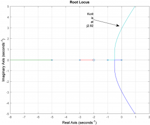
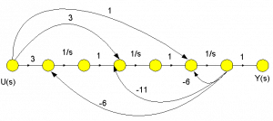
10.9.13 Example
Consider a certain unit feedback closed loop control system where the process is described by a transfer function [latex]G(s)[/latex]. We know that the process [latex]G(s)[/latex] is of a [latex]4th[/latex] order and that the process gain is equal to [latex]100[/latex]. Initially, the system is not compensated; i.e. the controller transfer function is [latex]G_{c}(s)=1[/latex]. Consider the Root Locus graph, taken for the uncompensated system, shown next. Based on the information in the graph, write the transfer function for the [latex]4th[/latex] order process [latex]G(s)[/latex] (Note – [latex]K[/latex] is the adjustable proportional gain used to obtain the Root Locus) and identify the system TYPE.

Now consider the same uncompensated system Root Locus with additional information obtained using MATLAB rlocfind function. Based on it, identify the critical gain that will cause the closed loop uncompensated system to be marginally stable, as well as the frequency of resulting oscillations.
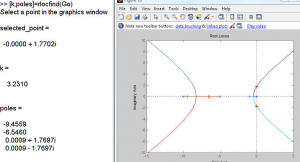
Now consider the compensated system Root Locus with information provided in the next graph, again obtained using rlocfind.

First, compare it with the uncompensated Root Locus and identify the type of Controller used, and its time constant, if it applies. Consider the compensated system Root Locus and identify the critical gain that will cause the closed loop compensated system to be marginally stable, as well as the frequency of resulting oscillations. Has the relative stability of the system improved after this Controller was implemented, or worsened? Explain.
10.9.14 Example
A certain process [latex]G(s)[/latex] is to work in a closed loop control system under Proportional Control [latex]K[/latex] in a unit feedback configuration. The process transfer function is described as follows:
[latex]G(s)= \frac{1}{s(s+1)(s+3)(s+3)}[/latex]
Find the closed loop system Characteristic Equation and determine the range of Proportional Gains [latex]K[/latex] for a stable closed loop system response, the critical value of gain at which the system would be marginally stable, and the resulting frequency of constant oscillations. Sketch a detailed, to-scale, root locus of the closed loop system poles for [latex]0
10.9.15 Example
Consider the feedback system under Proportional Control as shown:
[latex]G_{open}(s) =K\cdot G(s)=K\cdot \frac{10}{s(s+6)(s+10)}[/latex]
Sketch a detailed, to-scale, Root Locus of the closed loop system poles for [latex]0
10.9.16 Example
Consider the feedback system under Proportional Control as shown:
Find its transfer function. The system will work in a closed loop feedback configuration with a unity feedback and under Proportional Control (Gain [latex]K[/latex]). Find the closed loop transfer function of the system,[latex]G_{cl}(s)=\frac{Y(s)}{R(s)}[/latex], and establish the range of positive gain [latex]K[/latex] values that would result in a stable closed loop system response by using the Root Locus. Find the critical gain [latex]K_{crit}[/latex], at which the system would be marginally stable, and the corresponding frequency of oscillations of the marginally stable response [latex]\omega_{osc}[/latex].
10.9.17 Example
Consider a closed loop unit feedback system, where the process transfer function is as follows:
[latex]G(s)=\frac{1}{s(s+1)(s+2)}=\frac{1}{s^3+3s^2+2s}[/latex]
Assume that the compensated system will work under Proportional Control and find the controller setting such that Percent Overshoot will be [latex]+10\%[/latex].
10.9.18 Example
An actuator/process in a unit feedback closed loop control system. First, consider Proportional Control and find the gain value such that the PO is approximately [latex]+20\%[/latex]. What is the Settling Time? Can it be improved?
Next, a Parallel PID controller is added to the feed-forward path of the system.
Find controller parameters so that the closed loop system has: a pair of dominant poles with a time constant of 1 second and the actual frequency of oscillation of [latex]2[/latex] rad/sec and a pole with time a constant of [latex]0.1[/latex] second.
10.9.19 Example
Consider a unit feedback control system under PID Control, where the process transfer function is described below as [latex]G(s)[/latex], and the PID Controller transfer function is described below as [latex]G_{PID}(s)[/latex] :
[latex]G(s)=\frac{10}{s^2+10s+24}[/latex]
[latex]G_{PID}(s)=K_p(\frac{1}{\tau_is}+1)(\tau_ds+1)[/latex]
Where [latex]\tau_i = 0.5[/latex] seconds and [latex]\tau_d = 0.05[/latex] seconds. Sketch a detailed Root Locus for the system, including crossovers with the Imaginary axis, if any, break-away/break-in coordinates, if any, asymptotes, if any, centroid, etc. If you are using estimates, explain how you arrived at them. It is desired that the compensated closed loop system step response has an equivalent damping ratio equal to [latex]0.6[/latex] – assume that the closed loop system can be approximated by a second order model based on the dominant pair of complex poles and determine the appropriate value of the Proportional Gain [latex]K_p[/latex] for the PID Controller. Briefly discuss why the assumption made in Item [latex]2[/latex] is justified. Next, determine the [latex]2nd[/latex] order model parameters [latex]K_{dc}[/latex], [latex]\zeta[/latex], and [latex]\omega_n[/latex] to accurately describe the compensated closed loop system, and write the model transfer function [latex]G_m(s).[/latex]What are your estimates of the Percent Overshoot, PO, Settling Time, [latex]T_{settle(\frac{+}{-}2)}[/latex], and Steady State Error, [latex]e_{ss(\%)},[/latex] in the closed loop step response? NOTE: you can solve this item without having a complete solution to Item [latex]2[/latex].
10.9.20 Example
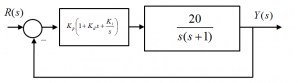
Consider a unit feedback control system that is open-loop unstable, where the process transfer function [latex]G(s)[/latex] is described as:
[latex]G(s)=\frac{10}{s(s+20)(s-1)}[/latex]
Determine if it is possible to stabilize the closed loop system by using Proportional Control only – to do so, sketch a Root Locus for the uncompensated system. Provide only rough estimates of any break-away/break-in coordinates. Use the Root Locus plot to justify your answer, very briefly.
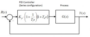
To stabilize the system, a series configuration of a PID Controller and a PI Controller with Rate Feedback are considered, as shown in the following diagrams. In both cases, the Controller Time Constants are: [latex]T_i=2[/latex] seconds and [latex]T_d=5[/latex] seconds. The closed loop Characteristic Equation is the same for both implementations:
[latex]1+K_p(1+\frac{1}{T_is})(1+T_ds)G(s)=0[/latex]
[latex]1+\frac{5K_p(s+0.5)(s+2)}{s^2(s+20)(s-1)}=0[/latex]

The resulting Root Locus plot will be the same for both compensation schemes. Sketch the Root Locus – provide only rough estimates of break-away/break-in coordinates. To save time, the Routh-Hurwitz Stability Criterion results have already been computed for you: [latex]K_{crit}[/latex] = 6.36 V/V and [latex]\omega_{osc}[/latex] =2.05 rad/sec.
Next, assume a dominant complex poles model for the compensated closed loop system – see transfer function [latex]G_m(s)[/latex]– and use the Root Locus sketch to choose the location corresponding to the Settling Time,[latex]T_{settle(\pm2\%)}[/latex], equal to 2 seconds. Calculate the corresponding Proportional Gain [latex]K_p[/latex]. What is the expected Percent Overshoot and Steady State Error in the closed loop step response?
Part 3: If the Series PID Controller Configuration is implemented, will the actual Settling Time and Percent Overshoot differ from the values expected based on the dominant poles model? If so, why? No calculations required – answer very briefly.
If the PI + Rate Feedback Controller Configuration is implemented, will the actual Settling Time and Percent Overshoot differ from the values expected based on the dominant poles model? If so, why? No calculations required – answer very briefly.
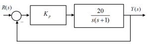
10.9.21 Example
Consider a closed loop control system working in a unit feedback configuration under Proportional Control, where the process transfer function is described as follows:
[latex]G(s) = \frac{10}{(s+2)^2(s+10)}[/latex]
Part 1. Sketch the root locus plot and calculate all relevant coordinates, such as the crossovers through the Imaginary Axis, the break-away, the centroid and the asymptotic angles.
Part 2. Determine the value of the Operational Gain ([latex]K_{op}[/latex]) such that the closed loop step response will have a Percent Overshoot of 5%. For the computed value of the Operational Gain, [latex]K_{op}[/latex] , answer these questions:
- What will be the steady state error, in [latex]\%[/latex], of the closed loop step response?
- What will be the Settling Time, [latex]T_{settle(\pm2\%)}[/latex] of the closed loop step response?
- What will be the system Gain Margin?
10.9.22 Example
Consider the feedback system under Proportional Control as shown:
[latex]G_{open(s)} = K[/latex] ⋅ [latex]G(s) =[/latex] [latex]K[/latex] ⋅ [latex]\frac{s+8}{s(s+6)(s+10)}[/latex]
Sketch a detailed Root Locus for the system, including crossovers with the imaginary axis, if any, break-away/break-in coordinates, if any, asymptotes, if any, a centroid, etc. if you are using estimates, explain why.
Determine the value of the gain [latex]K_{p}[/latex] that would result in the closed loop system equivalent damping ratio of [latex]\zeta = 0.707[/latex] . What is the system Gain Margin at this value of the gain?
Find the closed loop transfer function at the gain as calculated. Would the system closed loop behaviour be well approximated by a second order model at this gain setting? Briefly justify your answer. If it is yes, determine the remaining model parameters [latex]K_{dc}[/latex] and [latex]\omega_n[/latex] , and write the model transfer function [latex]G_{m(s)}[/latex]. What will be the expected Percent overshoot, Settling Time and Steady State Error of the closed loop step response?
10.9.23 Example
Consider a unit feedback control system under Proportional Control, where the process G(s) is described by a different transfer function:
[latex]G(s) = \frac{1}{(s-5)(s^2 +6s+40)}[/latex]
Note that the process [latex]G(s)[/latex] is unstable and that it also has a pair of complex poles. Your task is to investigate the behaviour of the closed loop system, including its stability, using Root Locus Analysis. Sketch a detailed Root Locus for the system, including break-away/break-in coordinates, if any, asymptotes, if any, a centroid, angles of departure from the complex poles, etc. If you are using estimates, explain why. Determine the exact coordinates of the crossovers of the Root Locus with the Imaginary Axis. Next, determine the value(s) of the Proportional Controller Gain, [latex]K_{p}=K_{crit}[/latex] , at which the closed loop system becomes marginally stable, and the corresponding frequency(ies) of marginally stable oscillations, [latex]\omega_{osc}[/latex] . Finally, determine the practical range of safe operating gains for the Proportional Controller in this system.
10.9.24 Example
Consider a certain closed loop unit feedback control system under Proportional + Derivative Control with Derivative Time Constant [latex]\tau_{d}[/latex] = 2 where the Controller and the Process G(s) are described as follows:
[latex]G_{c}(s) = K_{p}(1+T_{d}s)[/latex] [latex]G(s)[/latex] = [latex]\frac{2}{s^2(s+5)}[/latex]
Part 1: Sketch a Root Locus plot of the system. Find all relevant coordinates, including its centroid, asymptotic angles, if any, accurate coordinates of the break-away/break-in points, if any, accurate coordinates of crossovers with the Imaginary Axis, if any.
Part 2: Use the Root Locus sketch to select a PD Controller Gain [latex](K_{p})[/latex] such that the closed loop system would have the damping ratio of the dominant complex poles equal to [latex]\zeta = 0.707[/latex]. Note that there are two possible choices of the Controller Gain that meet the [latex]\zeta[/latex] condition – clearly indicate their location on the Root Locus, then select the location that would result in a more desirable response and calculate the corresponding PD Controller Gain, [latex]K_{p}[/latex].
Briefly justify your choice of the Root Locus location for the Controller gain.
Part 3: Estimate the following compensated closed loop response specifications when the PD Controller Gain value is as chosen in Part 2: PO, [latex]T_{settle(\pm2\%)}[/latex], [latex]e_{ss(step\%)}[/latex], [latex]e_{(ramp)}[/latex], [latex]e_{ss(parab)}[/latex].
