Chapter 5
5.2 Steady State Error Analysis in an Equivalent Unit Feedback Loop
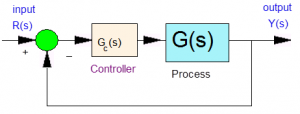
Consider a unit feedback loop system shown in Figure 5‑4. Note that typically a system does NOT have a unit feedback – this configuration is a result of an equivalent manipulation of the block diagram as shown above.
The system error was defined in Equation 5‑2. Assume the open loop transfer function of the system to be in a polynomial form as shown in Equation 5‑3 where N – number of integrators (poles at the origin) in the open loop transfer function, is called the system type. System type affects the steady state accuracy of the system response.
| [latex]G_C(s)G(s)=G_{open}(s)[/latex]
[latex]G_{open}(s)=\frac{N(s)}{s^NQ_1(s)}[/latex] |
Equation 5‑3 |
If the system is stable, then the Final Value Theorem applies:
| [latex]e_{ss}=lim e(t)=lim_{s\mapsto 0 }sE(s)[/latex]
[latex]E(s)=R(s)-Y(s)=R(s)-R(s)G_{closed}(s)=R(s).\left ( 1-\frac{G_{open}(s)}{1+G_{open}(s)} \right )[/latex] [latex]E(s)=R(s)\frac{1}{1+G_{open}(s)}[/latex] [latex]e_{ss}=lim_{s\mapsto 0 }sE(s)=lim_{s\mapsto 0 }s.R(s).\frac{1}{1+G_{open}(s)}[/latex] [latex]e_{ss}=lim_{s\mapsto 0 }sR(s).\frac{1}{1+\frac{N(s)}{s^NQ_1(s)}}[/latex] |
Equation 5‑4 |
5.2.1 Steady State Error for a Step Input
The steady state error can now be evaluated for three Standard Power-of-Time Inputs: step, ramp and parabola. Let’s start with a step input:
| [latex]r(t)=1(t)\Rightarrow R(s)=\frac{1}{s}[/latex]
[latex]e_{ss}=lim_{s\mapsto 0 }sR(s).\frac{1}{1+\frac{N(s)}{s^NQ_1(s)}} =[/latex] [latex]lim_{s\mapsto 0 }s\frac{1}{s}.\frac{1}{1+\frac{N(s)}{s^NQ_1(s)}}=[/latex] [latex]lim_{s\mapsto 0 }\frac{1}{1+\frac{N(s)}{s^NQ_1(s)}}[/latex] |
Equation 5‑5 |
Define the position error constant:
| [latex]k_{pos}=lim_{s\mapsto 0 }G_{open}(s)=lim_{s\mapsto 0 } \frac{N(s)}{s^NQ_1(s)}[/latex] | Equation 5‑6 |
The steady state error is then:
| [latex]e_{ss}=lim_{s\mapsto 0 }\frac{1}{1+\frac{N(s)}{s^NQ_1(s)}} =\frac{1}{1+K_{pos}}[/latex] | Equation 5‑7 |

Note on the plots, that while tracking in the Steady State improves as the system type goes up (i.e. the Steady State Error is reduced), the transient response of the system is becoming more and more oscillatory. This is the result of the presence of integrators (one for System Type One, and two for System Type Two). The more integrators in a closed loop, the more difficult it is for the system to maintain stability. That is why we don’t use control systems of Type higher than Two.
An important observation here, that we will return to later, is that presence of integrators reduces the relative stability of a system, i.e. reduces the system Gain Margin.
5.2.2 Steady State Error for a Ramp Input
Check Laplace Tables entry for a ramp input:
| [latex]r(t) = t. 1(t) \rightarrow R(s) = \frac{1}{s^{2}}[/latex]
[latex]e_{ss} = lim_{s\mapsto 0 } s. R(s). \frac {1}{1+\frac{N(s)}{s^{N}Q_{1}(s)}} =[/latex] [latex]lim_{s\mapsto 0 } s. \frac{1}{s^{2}}. \frac{1}{1+\frac{N(s)}{s^{N}Q_{1}(s)}} = lim_{s\mapsto 0 }\frac{1}{s+\frac{N(s)}{s^{N-1}Q_{1}(s)}}[/latex] |
Equation 5‑8 |
Define the velocity error constant:
| [latex]K_{v} = \lim_{s\mapsto 0 }sG_{open}(s) = \lim_{s \to 0} \frac{N(s)}{S^{N-1}Q_{1}(s)}[/latex] | Equation 5‑9 |
The steady state error is then:
| [latex]e_{ss} =\lim_{s\mapsto 0 } \frac{1}{s + \frac{N(s)}{s^{N-1}Q_{1}(s)}} = \frac{1}{K_{v}}[/latex] |
Equation 5‑10 |
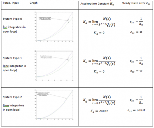
5.2.3 Steady State Error for a Parabolic Input
Check Laplace Tables entry for a ramp input:
| [latex]r(t) = \frac{1}{2}t^{2}. 1(t) \rightarrow R(s) = \frac{1}{s^{3}}[/latex]
[latex]e_{ss} = \lim_{s\mapsto 0 } s.R(s). \frac{1}{1+\frac{N(s)}{s^{N}Q_{1}(s)}} =[/latex] [latex]\lim_{s\mapsto 0 } s.\frac{1}{s^{3}}. \frac{1}{1+\frac{N(s)}{s^{N}Q_{1}(s)}} =[/latex] [latex]\lim_{s\mapsto 0 }\frac{1}{s^2+\frac{N(s)}{s^{N-2}Q_{1}(s)}}[/latex] |
Equation 5‑11 |
Define the velocity error constant:
| [latex]K_{pos} =\lim_{s\mapsto 0 } s^2G_{open}(s) =\lim_{s\mapsto 0 } \frac{N(s)}{S^{N-2}Q_{1}(s)}[/latex] |
Equation 5‑12 |
The steady state error is then:
| [latex]e_{ss} =\lim_{s\mapsto 0 } \frac{1}{s^2 + \frac{N(s)}{s^{N-2}Q_{1}(s)}} = \frac{1}{K_{a}}[/latex] |
Equation 5‑13 |