2.4 Determining Stable Range for Proportional Controller Operations

Consider a closed loop system under Proportional Control in Figure 2‑2:

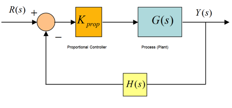
The closed loop transfer function and the system Characteristic Equation are:

The variable parameter – the Proportional Controller Gain – is now a part of the system Characteristic Equation and will feature in the Routh Array. This allows us to define the required condition for a stable, safe, range of Controller operations.

 Example

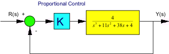
Consider the following control system:

• Is this system open-loop stable?
• Determine a range of gains K required for a stable operation of this closed loop system.

Solution:

Part 1: Open Loop

Open loop characteristic equation is:

[latex]Q(s) = s^{3}+ 11s^{2}+ 38s+ 4 = 0[/latex]

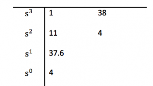
The system is open-loop stable, based on the Routh-Hurwitz Stability Criterion. We can also find numerically (MATLAB), what the poles of the open system are: -5.45 +j2.68, -5.45 – j2.68, -0.11.

The system Open Loop Transfer Function components are:

[latex]G(s)=\frac{4K_{prop}}{s^{3} +11s^{2}+ 38s+ 4},  H(s) = 1[/latex]

Part 2: Closed Loop

The system Closed Loop Transfer Function is:

[latex]G_{cl} = \frac{G(s)}{1 +G(s)H(s)}=\frac{\frac{4K_{prop}}{s^{3}+ 11s^{2}+ 38s +4}}{1 +\frac{4k_{prop}}{s^{3} +11s^{2}+ 38s+ 4}} = \frac{4K_{prop}}{s^{3}+ 11s^{2} +38s +(4K_{prop} +4)}[/latex]

Apply the Routh-Hurwitz criterion to the closed loop characteristic equation:

[latex]s^{3} +11s^{2}+ 38s +(4K_{prop}+ 4) = 0[/latex]

The Necessary Condition is:

[latex]4 +4K_{prop} > 0,   K_{prop} >-1[/latex]

The Sufficient Conditions from Routh Array:

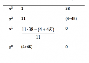
The resulting conditions are:

[latex]\frac{11\cdot 38 - (4+ 4K_{prop})}{11} > 0,  4K_{prop} < 414,  K_{prop} < 103.5[/latex]

The total condition is: [latex]-1 < K_{prop} < 103.5[/latex]

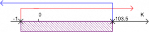
Note that the practical range of stable controller operations, as opposed to the previous purely mathematical condition, is [latex]0Critical Gain values. Again, of practical interest is only the upper, positive Critical gain value. What happens when the Controller gain reaches that Critical gain value?

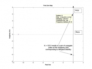
When [latex]K_{prop} = 103.5[/latex] :

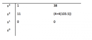
[latex]Q_{aux}(s) = 11s^{2} +418[/latex]

[latex]Q_{aux}(s) = 0[/latex]

[latex]s^{2} +38 = 0[/latex]

[latex]s_{1} = j\sqrt{38} = j6.16[/latex]

[latex]s_{2} = -j\sqrt{38} = -j6.16[/latex]

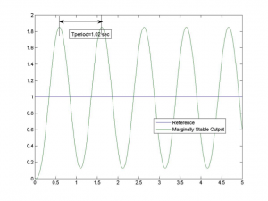
As the pole-zero map illustrates, the location of marginally stable poles on the Imaginary axis corresponds to the frequency of sustained oscillations, \[latex]\omega_{crit} = 6.16 rad/sec[/latex]. This corresponds to the period of oscillations equal to 1.02 seconds. Step response of the system when [latex]K_{prop}=103.5[/latex] is also shown.