
Chapter 11
11.3 Examples
11.3.1 Example
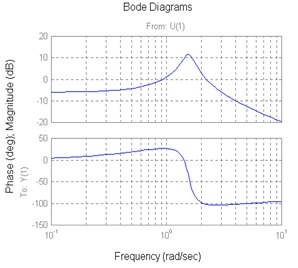
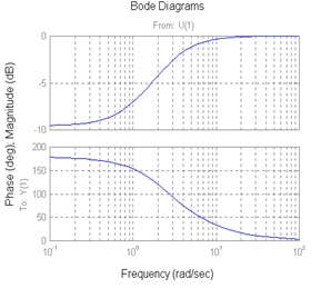
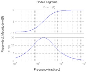
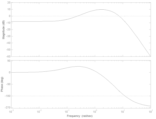
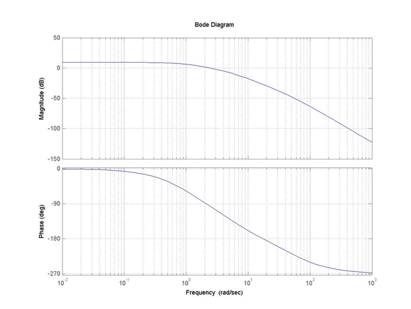
Let’s review the basics of Bode plots. A certain system has the following transfer function:
[latex]G(s)=\frac{(s+1)(s-2)}{(s+2)(s+3)}[/latex]
Match it with one of the Bode plots shown 6 below, A, B, C, or D, and clearly indicate your choice here.
 |
 |
 |
 |
11.3.2 Example
11.3.3 Example
[latex]G(s)=\frac{s+100}{(s+2)^{2}}[/latex]
Draw a Bode plot, i.e. a linear approximation, of its frequency response. Verify using Matlab, if the shape is correct.
11.3.4 Example
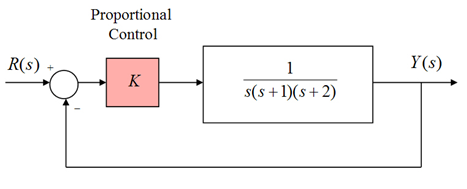
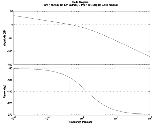
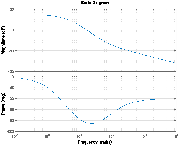
Consider again the closed loop unit feedback control system under Proportional Control (gain [latex]k_{p}[/latex]), discussed in Example 10.9.3. Open loop frequency response plots of the system (with [latex]k_{p}=1[/latex] are shown below.

Using the plots, find the system Gain Margin, Phase Margin and corresponding crossover frequencies. Determine the critical value of the gain, [latex]k_{crit}[/latex] , at which the system becomes marginally stable, and the corresponding frequency of marginally stable oscillations, [latex]\omega_{osc}[/latex] . Determine the range of gains [latex]k_{p}[/latex] to provide a stable closed loop system response. How do they compare to the solutions obtained in Example 10.9.3, based on the Routh-Hurwitz Criterion?
11.3.5 Example
11.3.6 Example
A certain unit feedback control system operates under Proportional Control (K is an adjustable gain). The process transfer function G(s) is not known. The following figure shows measured frequency response plots of the process, with linear approximations, i.e. the Bode Plot, already superimposed. Determine the transfer function of the process.
Next, use the accurate frequency response plots to determine the closed loop system Gain Margin [latex]G_{m}[/latex] and Phase Margin [latex]\Phi _{m}[/latex], and the corresponding crossover frequencies. Is the closed loop system stable? What is the critical gain, [latex]K _{crit}[/latex], at which the system will be marginally stable? What is the frequency of oscillations, [latex]\omega _{osc}[/latex], at that gain?
Finally, use the Routh-Hurwitz criterion to find the critical gain, [latex]K _{crit}[/latex], at which the system will be marginally stable, and the frequency of oscillations, [latex]\omega _{osc}[/latex], at that gain. Are the results of items a) and b) the same? Explain any discrepancies.

11.3.7 Example
Consider the following process transfer function of a unit feedback control system:
[latex]G(s)=\frac{10(3s+1)}{3s(s^{2}+5s+6)(s^{2}+2s+1)}[/latex]
Assume the Proportional Control and find the stability range for this system using Routh-Hurwitz Criterion, Root Locus and then Gain Margin from Bode plot. Note that for the latter, you need to sketch the plot first.
11.3.8 Example
Consider a unit feedback system under Proportional Control, where G(s) is a transfer function of an unknown process. Frequency response of the process was measured and its plots are shown next. Use the accurate frequency response plots to determine the Gain Margin of the system, the corresponding frequency of crossover, and the maximum value ([latex]K_{crit}[/latex]) of the gain range for a stable operation of the closed loop system. Next, use the linear approximations of the magnitude plot (also shown) to identify the process transfer function G(s) – the process is known to be minimum phase. Form the Routh Array and apply the Routh-Hurwitz criterion to determine the range of gains for the stable operation of the closed loop system as well as the frequency at which the system response will oscillate if the gain is set to its maximum value ([latex]K_{crit}[/latex]).

11.3.9 Example
Consider again the control system discussed in Chapter 2.4, where we had a unit feedback system under Proportional Control:
[latex]G_{open}(s)=K.G(s)=K.\frac{4}{s^{3}+11s^{2}+38s+4}[/latex]
Determine the range of gains K required for a stable operation of this closed loop system using the Gain Margin from frequency response. Recall that the critical gain was found from the Routh-Hurwitz Criterion to be [latex]K_{crit}=103.5[/latex], and from the Auxiliary Equation, we found [latex]\omega _{osc}=6.16[/latex] rad/sec.
11.3.10 Example
An open loop transfer function of a certain unit feedback control system is described as follows:
[latex]G_{open}(s)=K.G(s)=K.\frac{100}{(s+1)^{2}(s+10)}[/latex]
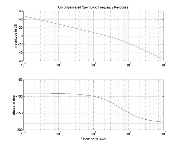
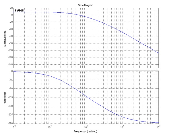
K is an adjustable gain and G(s) is the process transfer function. On the graph provided, plot a straight-line approximation of the magnitude and phase of the transfer function, [latex]G_{open}(j\omega)=K.G(j\omega)[/latex], for K=10. From your plot, measure the relative stability of the closed loop system by finding the system Gain Margin, GM, the Phase Margin, PM, the corresponding crossover frequencies, and the range of positive gain K for a stable operation of the closed loop system. Apply the Routh-Hurwitz criterion of stability to this system to find the range of positive gain K that ensures stable operation of the closed loop. Briefly outline reasons for any discrepancy with your results.
11.3.11 Example
Consider a unit feedback system under Proportional Control:
[latex]G_{open}(s)=K.G(s)=K.\frac{20}{(s+1)^{2}(s+2)(s+3)}[/latex]
Find the system Gain Margin, Phase Margin and corresponding crossover frequencies. Determine the critical value of the gain, [latex]K_{crit}[/latex], at which the system becomes marginally stable, and the corresponding frequency of marginally stable oscillations, [latex]\omega_{osc}[/latex]. Determine the range of gains [latex]K_{p}[/latex] to provide a stable closed loop system response.
Verify the results from Part A by applying the Routh-Hurwitz Criterion of Stability: find the critical value of the gain, [latex]K_{crit}[/latex], at which the system becomes marginally stable, and the corresponding frequency of marginal oscillations, [latex]\omega_{osc}[/latex]. Comment on discrepancies, if any.
11.3.12 Example
Consider a unit feedback system under Proportional Control:
[latex]G_{open}(s)=K.G(s)=K.\frac{30}{(s+1)^{2}(s+2)(s+5)}[/latex]
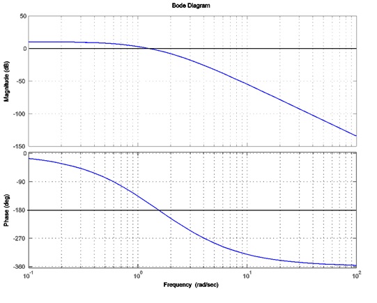
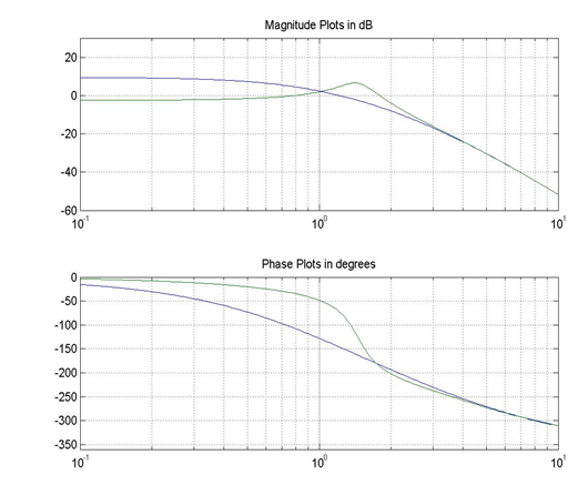
Frequency response plots of the open and closed loop (assuming Controller Gain [latex]K_{op}[/latex] = 1) are shown below – NOTE: the plots are not labelled – you should be able to recognize which plot corresponds to which response.
Using the open loop frequency response plot, apply Bode Criterion of Stability. Verify the above results by applying the Routh-Hurwitz criterion of Stability. Compute the critical value of the gain, [latex]K_{crit}[/latex], that would result in a marginal stability of the system, and the frequency of resulting marginal oscillations, [latex]\omega_{osc}[/latex]. Explain any possible sources of discrepancies.
11.3.13 Example
Consider a unit feedback system under Proportional Control, as shown. Frequency plots of the system open loop are also shown.
Find the system Gain Margin, Phase Margin and corresponding crossover frequencies. Determine the critical value of the gain, [latex]K_{crit}[/latex], at which the system becomes marginally stable, and the corresponding frequency of marginally stable oscillations, [latex]\omega_{osc}[/latex]. Determine the range of gains [latex]K_{p}[/latex] to provide a stable closed loop system response. Use MATLAB functions “margin” and ” rlocfind” to verify these results.
Verify the results from Part 1 by applying the Routh-Hurwitz Criterion of Stability: find the critical value of the gain, [latex]K_{crit}[/latex], at which the system becomes marginally stable, and the corresponding frequency of marginally stable oscillations, [latex]\omega_{osc}[/latex].
11.3.14 Example
Consider a unit feedback system under Proportional Control, as shown. Frequency plots of the system open loop transfer function when the operational gain is [latex]K_{op}[/latex] = 1 are shown next.

Apply the Bode stability criterion (i.e. determine the closed loop system Gain Margin, Phase Margin and the corresponding crossover frequencies) for two cases, when the operational gain is [latex]K_{op}[/latex] = 1 and [latex]K_{op}[/latex] = 10.
Apply the Routh-Hurwitz stability criterion to this system and determine the critical value(s) of gain, [latex]K_{crit}[/latex] for system stability, as well as the frequency of oscillations, [latex]\omega_{osc}[/latex], resulting when [latex]K=K_{crit}[/latex]. Next, assuming that the operational values of the proportional gain are again [latex]K_{op}[/latex] = 1 and [latex]K_{op}[/latex] = 10, compute the corresponding values of the Gain Margins. Comment if the results you get are consistent with the results from item # 1.
Next, find the range of operational gains [latex]K_{op}[/latex] such that the system is stable AND the steady state error to the unit step reference signal is less than 10%. When the error is exactly 10%, what is the system Gain Margin? Is it possible to operate the closed loop system that the steady state error requirement is no more than 5%? If yes, why? If no, why?
11.3.15 Example
Consider a unit feedback system under Proportional Control, as shown. Frequency plots of the system open loop transfer function when the operational gain [latex]K_{op}[/latex] is = 1 are shown next. Apply the Bode stability criterion for two cases, when [latex]K_{op}[/latex] = 1 and [latex]K_{op}[/latex] = 10, verify using Routh Array.
11.3.16 Example
Consider a certain closed-loop unit feedback control system under Proportional Control (gain ) where the process transfer function is as follows:
[latex]G(s)=\frac{(s+50)(s+100)}{(s+2)(s+4)(s+10)}[/latex]
Sketch a Root Locus plot of the system. However, only very rough estimates of break-in and break-away points are required (no calculations) – focus on the overall shape of the plot and on the crossovers with the Imaginary Axis. Determine the critical value (or values) of the gain,[latex]K_{crit}[/latex], at which the system is marginally stable, and the corresponding frequency (or frequencies) of marginally stable oscillations,[latex]\omega_{osc}[/latex] . Use the Root Locus plot to interpret the results and to correctly determine the range (or ranges) of the gains [latex]K_{p}[/latex] that will provide a stable closed loop system response. A frequency response plot of G(s) is provided – use the plot to verify the above results – to do so, clearly identify the frequency (or frequencies) of marginally stable oscillations, [latex]\omega_{osc}[/latex], and the corresponding values of the gain, [latex]K_{crit}[/latex].
Verify the stability results using Routh Array and Routh-Hurwitz Criterion of stability.
11.3.17 Example
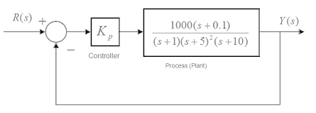
Consider a certain unit feedback closed-loop control system under Proportional Control, as shown. Open-loop frequency response plots of the system with [latex]K_{p}=1[/latex]are shown as well.
[latex]G_{open}(S)=K.G(s)=K.\frac{100}{s(s+5)^{2}}[/latex]
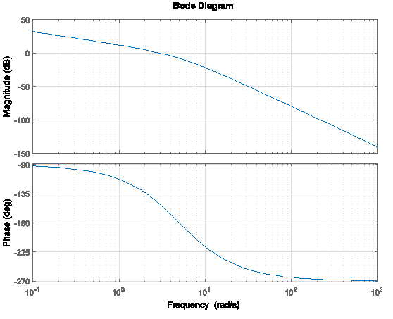
Using the plots, find the system Gain Margin, Phase Margin, and corresponding crossover frequencies. Determine the critical value of the gain, [latex]K_{crit}[/latex], at which the system becomes marginally stable, and the corresponding frequency of marginally stable oscillations, [latex]\omega_{osc}[/latex]. Determine the range of gains [latex]K_{p}[/latex] to provide a stable closed-loop system response.
Verify the results above by applying the Routh-Hurwitz Criterion of Stability: find the critical value of the gain, [latex]K_{crit}[/latex] at which the system becomes marginally stable, and the corresponding frequency of marginally stable oscillations, [latex]\omega_{osc}[/latex]. How do they compare to item 1)? Part 3: For [latex]K_{p}=1[/latex], determine the following closed loop steady-state response specifications: System Type, Error Constants and Errors.
