Chapter 10
10.5 Evans Root Locus Construction Rule # 3: Asymptotic Angles and Centroid
This Rule deals with the asymptotic angles and centroid location. If gain K is large enough, one can see that the branches of the RL travelling towards infinity follow a straight-line path that is asymptotic to a hypothetical line, called an asymptote, at a certain angle, called an asymptotic angle. If one extended these hypothetical lines, they would all intersect at an “anchor” point, called a centroid. Evans showed that the asymptotic angles and the centroid location can be computed as shown in this Rule.
When the test point [latex]s^*[/latex] is close to the open loop singularities (poles, zeros), angles for vectors drawn from the singularity towards the point [latex]s^*[/latex] , which are used to evaluate [latex]G(s^*)[/latex] function, are quite different. However, as the gain K tends to approach infinity, [latex]K \rightarrow \infty[/latex], which is the descriptor for asymptotic condition, point [latex]s^*[/latex] begins to practically lie on the asymptote, and these angles all begin to look alike and approach the asymptotic angle [latex]\theta_i[/latex].
Recall that the total angle of the function [latex]G(s^*)[/latex] is equal to:
| [latex]\angle G(s^*)=\angle_{zeros}-\angle_{poles}[/latex] | Equation 10-7 |
The total angles, respectively, for all vectors associated with poles and all vectors associated with zeros, will be equal to:
| [latex]\angle_{poles} = n\cdot\theta_i[/latex] | |
| [latex]\angle_{zeros}=m\cdot\theta_i[/latex] | Equation 10-8 |
If the test point [latex]s^*[/latex] is to belong to the root locus, the angle of [latex]G(s^*)[/latex] has to meet the angle criterion:
| [latex]\angle G(s^*)=180^{\circ}[/latex] | |
| [latex]m\cdot\theta_i - n\cdot\theta_i=180^{\circ}[/latex] | Equation 10-9 |
In the formula below, the sign in the denominator is reversed, because [latex]m\leq n[/latex]. This will have no effect on the formula, because [latex]+180^{\circ}=-180^{\circ}[/latex]. The asymptotes need to be anchored on the plot. To do that, a so-called root locus centroid is defined, as a “centre of gravity” of the plot.
Rule 3: The asymptotes are centred on the Real axis at the centroid, described by this equation:
| [latex]\sigma = \frac{\sum poles - \sum zeros}{n-m}[/latex] | Equation 10-10 |
The branches of Root Locus that tend to infinity converge at asymptotic angles, described by this equation:
| [latex]\theta_i = \frac{180^{\circ}\pm k\cdot360^{\circ}}{n-m}[/latex] | [latex]k=0,1,...,(n-m-1)[/latex] | Equation 10-11 |
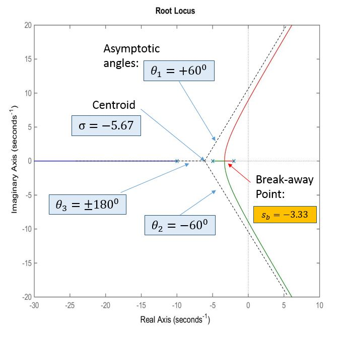
As an example, consider RL shown in Figure 10‑4. Centroid and asymptotes are calculated as follows:
[latex]\sigma = \frac{-10-5-2}{3-0}=-5.67[/latex], [latex]\theta_i = \frac{180^{\circ}\pm k\cdot360^{\circ}}{3-0}=60^{\circ},180^{\circ},-60^{\circ}[/latex]
See how this shows on the RL plot in Figure 10‑6.