8.6 The Effect of a Non-Minimum Phase Zero on the 2nd Order System Response

Let us consider a special case of a system with a zero in the RHP. Note that such a case has nothing to do with the system stability, as the stability is decided by the locations of poles only. A zero in the RHP is called a non-minimum phase zero (what follows is that the zero in the LHP is called a minimum-phase zero, to distinguish between the two). The name refers to the phase characteristics of the two singularities, as shown in Figure 8‑12 and Figure 8‑13.

Physical systems typically have several poles, each contributing a negative phase angle going from 0 degrees to -90 degrees as the frequency increases, and only one or two zeros. An LHP zero contributes a positive phase angle going from 0 degrees to +90 degrees as the frequency increases. Thus the effect of the LHP zero in the frequency domain is that the overall negative phase, or phase lag, decreases. In contrast, an RHP zero has a phase characteristic that is the opposite of the LHP zero, contributing a negative phase angle going from 0 degrees to -90 degrees as the frequency increases. Thus, the effect of the RHP zero in the frequency domain is that the overall negative phase, or phase lag, increases. When comparing two systems, one with the LHP zero, and one with the RHP zero, the overall phase angle characteristic of the latter one will be more negative than of the former one, hence the name, non-minimum phase. See an example in the next section for such a comparison.

Let us examine the effect of the RHP zero on the system transient response. Let’s assume that a standard second order system has an additional RHP zero at s = +a. The transfer function gain is adjusted to remain constant:

As before, the transfer function in Equation 8‑3 can be considered as a sum of two components – the first component is the standard second order model, and the second component acts as a derivative on the response signal. However, because the zero was in RHP, the magnitude of this component is negative.

Now consider its effect on the system response Y(s) to a unit step:

[latex]Y(s)=G_{mod}(s)\cdot R(s)=G_{mod}(s)\cdot\frac{1}{s}[/latex]

[latex]Y(s)=\Bigg \{ K_{dc}\cdot\frac{\omega_n^2}{s(s^2+s\zeta\omega_n s + \omega_n^2)} \Bigg \} - \frac{1}{a}\cdot s \Bigg \{K_{dc}\cdot\frac{\omega_n^2}{s(s^2+s\zeta\omega_n s + \omega_n^2)}\Bigg\}[/latex]

The above expression for the system response is again a superposition of two components: a step response of the standard second order model, and a derivative of the same step response, but with a negative multiplier 1/a. Depending on the magnitude of a, this component may be small or large. Thus, if a is large, i.e. the zero is far away in the RHP, the magnitude of this negative derivative term is insignificant and can be safely ignored. However, if the RHP zero is close to the Imaginary axis, the magnitude of this negative signal component rapidly increases. The superposition of a signal and its negative derivative creates not only an exaggerated Percent Overshoot, but also an initial negative “dip” in the system response. Such a dip is a tell-tale sign of a significant RHP zero. The zero cannot be ignored and has to be included in the system model.

Note that the presence of the non-minimum zero presents a control problem, because systems exhibiting non-minimum phase characteristics are difficult to improve on. The negative dip creates an effective time delay, thus increasing the rise time and the settling time. However, this issue cannot be easily addressed with Classic Control approaches – a good controller will reduce oscillations and shorten the settling time, but the effective lag will remain. Let’s consider a second order overdamped system with poles at -5 and -3, and an additional zero at a = +50:

[latex]G(s)= 0.85\cdot\frac{15}{(s+5)(s+3)}\cdot\frac{(-s+50)}{50}=\frac{-0.255s+12.75}{s^2+8s+15}[/latex]

The plot of its step response is shown in Figure 8‑14, compared to the response of a model without the zero. Again predictably, based on Equation 8‑2 there is virtually no effect on the system response of the zero far in the insignificant region (i.e. in the far positive magnitudes of RHP). If we were looking for a simpler model for this system, the zero can safely be ignored:

[latex]G_m(s)=0.85\frac{15}{s^2+8s+15}[/latex]

Now, let’s see what happens when the zero is moved into the significant region close to the dominant poles. Assume a  = +2. The plot is shown in Figure 8‑15. The magnitude of the negative derivative term in Equation 8‑2 is now much larger.  This will cause a very visible “dip,” or “Undershoot,“ at the beginning of the system response – the initial response initially goes negative. In some systems the change of polarity may not be acceptable, in others the problem is the effective delay created by the polarity reversal.

[latex]G(s)=0.85\cdot\frac{15}{(s+5)(s+3)}\cdot\frac{(-s+2)}{2}=\frac{-6.37s+12.75}{s^2+8s+15}[/latex]

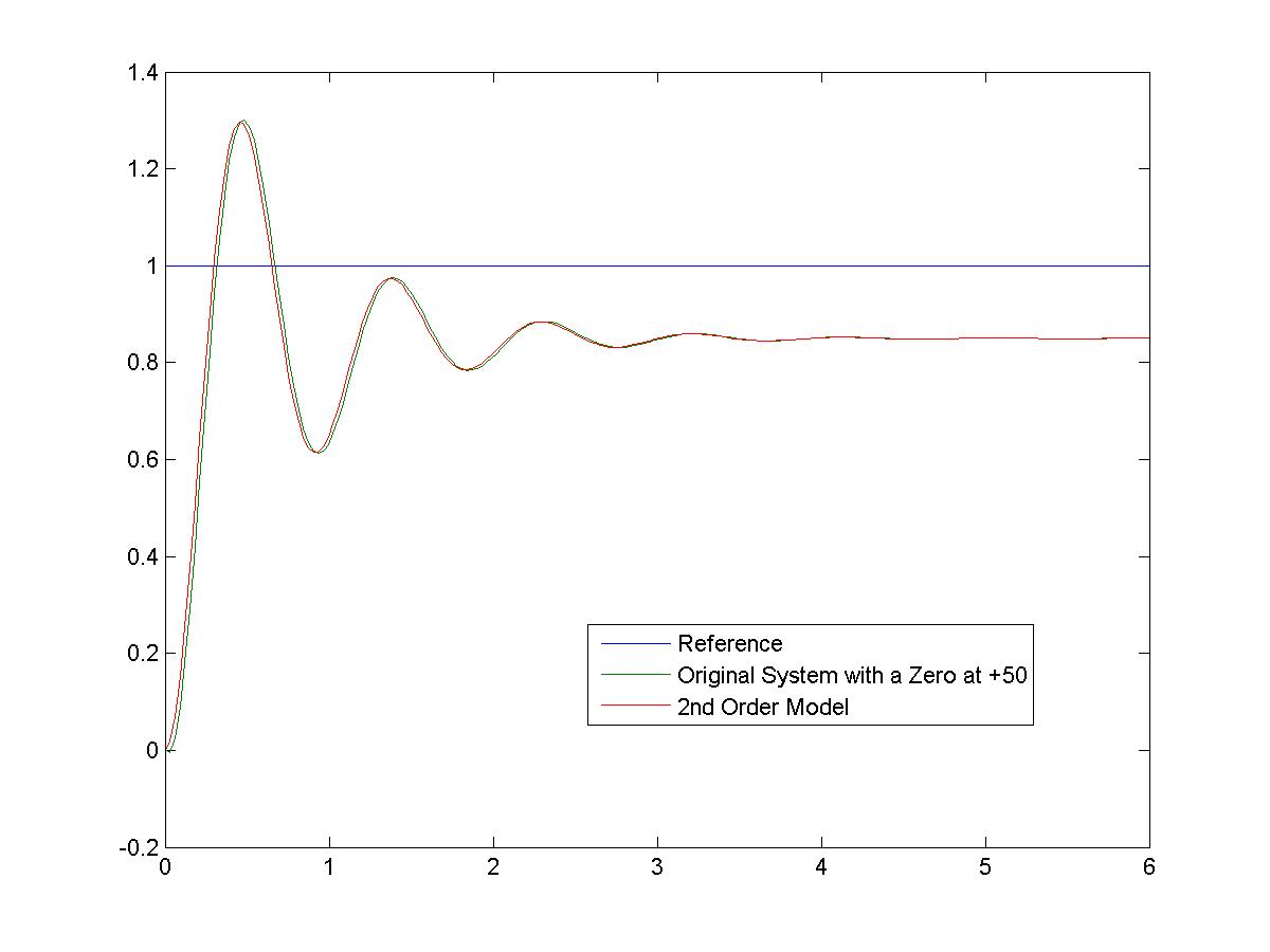
As a result of the delay, the Rise Time and Settling Time will be longer (worse). We would not be able to replace the system dynamic with a simplified model – the RHP zero has to be included in the description. Note that this “Undershoot” effect is a mirror image of what happens with a significant zero in the LHP in an overdamped system where an “artificial” Percent Overshoot was formed. Next, consider a second order system with a pair of complex poles is: [latex]s_1 = -1.4 + j6.86[/latex], [latex]s_2 = -1.4 - j6.86[/latex], and an additional zero at a = +50:

[latex]G(s)=0.85\cdot\frac{49}{(s^2+2.8s+49)}\cdot\frac{(-s+50)}{50}=\frac{-0.833s+41.7}{s^2+2.8s+49}[/latex]

The plot of its step response is shown in Figure 8‑16, compared to the response of a system without the zero added. Predictably, based on Equation 8‑2 there is virtually no effect on the system response of the zero far in the insignificant region, with the Undershoot and the resulting delay almost invisible. Note that when a zero is in an insignificant region, it doesn’t matter that the zero is in the RHP – instead of far to the left, as in LHP, the insignificant region will be far to the right, tending towards positive large magnitudes. If we were looking for a simpler model for this system, the zero can safely be ignored:

[latex]G_{mod}(s)=0.85\cdot\frac{49}{(s^2+2.8s+49)}[/latex]

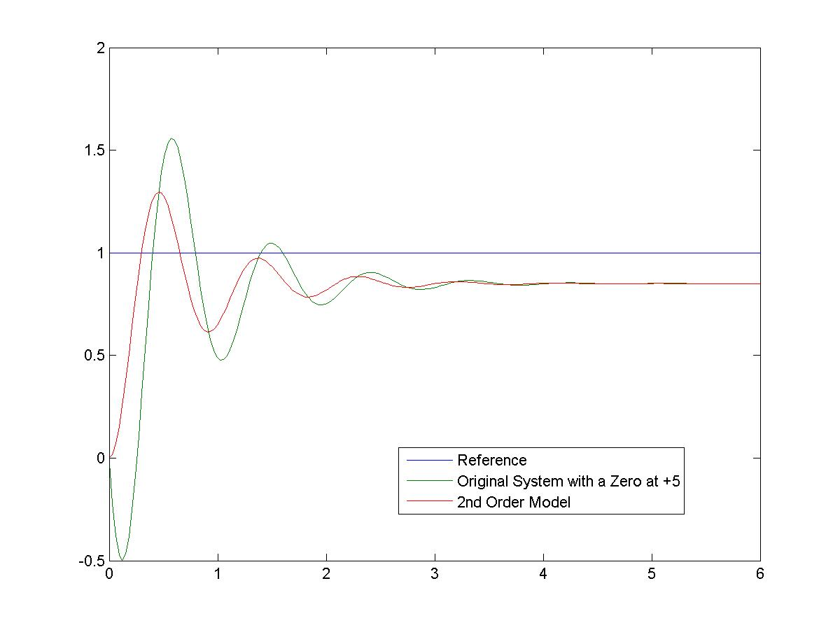
Now, let’s see what happens when the zero is moved into the significant region i.e. close to the Imaginary axis. Assume a = +5. The plot of its step response is shown in Figure 8‑17, compared to the response of a system without the zero added.

[latex]G(s)=0.85\cdot\frac{49}{(s^2+2.8s+49)}\cdot\frac{(-s+5)}{5}=\frac{-8.33s+41.7}{s^2+2.8s+49}[/latex]

The magnitude of the negative derivative term in Equation 8‑2 is now much larger.  This will cause a very visible Undershoot, or a dip, at the beginning of the system response – the initial response goes negative. As a result of the delay, the Rise Time and Settling Time will be longer (worse). The Percent Overshoot is again much worse (larger), as in the case of the zero in the LHP. The frequency of oscillations is not affected. We would not be able to replace the system dynamic with a simplified model – the RHP zero has to be included in the description.