
Chapter 9
9.1 Introduction
One of the most versatile controller configurations for simple single feedback loop control is a PID Controller. We already became familiar with the various forms of this controller both in the Lab as well as in two previous chapters, where we utilized the “Top-down” design approach to finding the controller gain values, based on the understanding of the second order model and the effects of additional poles and zeros on the system response. In this chapter, we will further discuss the properties of the three-mode controller (PID), including some of its practical aspects.

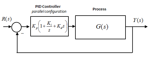
The three-mode-controller name (PID) stands for Proportional + Integral + Derivative. Its parallel configuration is realized as follows:
| [latex]G_{PID}(s)=K_p+\frac{K_i}{s}+K_d s[/latex] | |
| [latex] u(t)=K_p\cdot e(t)+K_i\int e(t)dt + K_d\frac{de(t)}{dt}[/latex] |
Equation 9‑1 |
where e(t) is error, and u(t) is the Controller output, actuating the Process. Equation 9‑1 represents the so-called Parallel PID Structure, where the three modes of controller operation are added – the controller output is a sum of the three control channels: P, I and D. The parallel structure is very easily implemented digitally. This form is also very convenient for intuitive, step-by-step controller tuning where each mode is added independently. For more on PID tuning, see appendices in Lab 2. The tuning approach, unlike the more analytical “top-down” design approach, does not guarantee the “best possible” combination of parameters, but it provides a good starting point for an analytical design where Root Locus Analysis or Frequency Response Analysis (more on Frequency Response to come in Chapter 12) are considered.
A variation of the Parallel Structure is also used, shown in Figure 9‑2, with the Proportional Controller Gain as a multiplier – it is more useful when Root Locus Analysis is used (more on Root Locus to come in Chapter 10), as we can vary the Proportional Gain – this is not possible for the classical Parallel Structure of Equation 9‑1.
However, the problem with the Parallel PID Structure is that the zeros of the closed loop transfer function, shown in Equation 9‑1, interact, since they are solutions of a quadratic term – when one zero location is changed (i.e. the value of one of the time constants is changed), the other zero moves as well.
Therefore, for a more analytical approach (i.e. if we want to use the Root Locus, or Frequency Response plots to design the PID Controller) this form is not so convenient: the two zeros interact, shifting at the same time. An alternative configuration of the PID Controller can be implemented, called the Series PID Controller Structure, shown in Figure 9‑3 and in Equation 9‑2. The zeros of the closed loop transfer function are now independent and can be moved on the Root Locus or on the Frequency Response plot one at a time.

| [latex]G_{PID}(s) = K_p(1+\frac{K_i}{s})(1+K_d s)[/latex] | Equation 9-2 |
Finally, when the Series PID structure is divided into two terms, one in the forward path and one in the feedback path, we have the PI + Rate Feedback structure as shown in Figure 9‑4.
Both the Parallel and the Series PID Structures have two zeros, and therefore contribute these two zeros to the closed loop transfer function. In case of the PI + Rate Feedback, only one zero is contributed to the closed loop transfer function. The PI + Rate Feedback Structure can be used if the Derivative effect has to be reduced because either we have a large additional overshoot in the step response because the system zeros are in the dominant region, or a wind-up effect is taking place, or when we are dealing with a noisy environment, since the Bandwidth of the system with only one zero is smaller than the Bandwidth of the system with two zeros and thus the configuration with the Rate Feedback provides more attenuation for noise, which is usually a higher frequency phenomenon.

In general, when dealing with a system under PID Control, we take the following steps:
- Obtain a closed loop system that is stable
- Exert a reasonable level of control signal to the process – the Proportional Controller does most of the work. Proportional Mode is the “work-horse”, or the “muscle”, of the PID Controller. Proportional Mode is used to provide a stable, fast and accurate response.
- Integral and Derivative Gains should be used sparingly, to make subtle adjustments in the system response:
- o Integral Mode increases the System Type and therefore reduces the steady state error – PI (Proportional + Integral) Control is used to improve steady state tracking.
- o Derivative Mode is used to increase damping – PD (Proportional + Derivative) Control is used to increase damping and therefore to decrease oscillations and also to speed up the system response.
- Fine-tune as required during implementation by adding the Integral and Derivative action.
An important observation about the PID Control – the Integral and Derivative action should be used sparingly! A nice analogy for the Controller settings is to think about the Proportional Control as the main meal, while the Integral and the Derivative are like salt and pepper – while these condiments are needed to have a tasty meal, too much of either will spoil the taste.
The basic control actions in a PID Controller are as follows:
- Proportional Control
- PI (Proportional + Integral) Control
- PD (Proportional + Derivative) Control (or its variation, Proportional + Rate Feedback)
- PID (Proportional + Integral + Derivative) Control
Plots in Figure 9-5 show the effects of the actions of each Controller Mode. Figure 9‑5 shows a screen capture of a Java Applet where a typical closed loop system response to Proportional Control is shown – steady state error vs. oscillation trade-off takes place as the gain is increased.
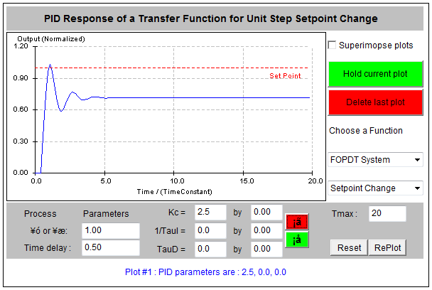
Figure 9‑6 shows the effect of PI Control, with the steady state error integrated to zero. Figure 9‑7 shows the effect of PD Control which has no effect on the steady state, but reduces oscillations in the transient state. Finally, Figure 9‑8 shows the effect of a well-tuned PID Controller.


