
Chapter 2
2.3 Stability in s-Domain: The Routh-Hurwitz Criterion of Stability
The original Criterion was formulated in a paper published in 1877 by Edward Routh, an English mathematician born in Upper Canada (now Quebec). In 1895 German mathematician Adolf Hurwitz formulated the Criterion in its today’s form, based on the theory of polynomials. This is why the Criterion bears both their names.
2.3.1 Necessary Condition for Stability
| Definition:
The Necessary Condition for Stability requires that all coefficients of the Characteristic Equation polynomial are present and have the same sign. |
In practice, it means that they should all be positive, as negative signs would correspond to a negative Controller gain. A control system with a negative gain is not practical as it would do exactly the opposite to the Command (Reference) input.
Where does the Necessary Condition come from? Consider the following. Once the Characteristic Equation is factorized into a ZPK form, it will consist of two types of factors, 1st and 2nd order, as shown. If the roots of these factors are in the LHP (i.e. the Stable Region of the s-plane), then the resulting coefficients in these factors will be positive:
[latex](s + a_{j})[/latex]
[latex](s^{2} + a_{k}s + b_{k})[/latex]– stable factors
For example [latex](s+5)[/latex] and [latex](s^{2} + 3s + 14)[/latex] are factors corresponding to stable pole locations (-5 and -1.5+j3.43, -1.5-j3.43, respectively), while [latex](s-5)(s^{2} - 3s + 14)[/latex], are factors corresponding to unstable pole locations (+5 and +1.5+j3.43, +1.5-j3.43 respectively). Also note that one of the two poles corresponding to the [latex](s^{2} + 3s - 14)[/latex]factor is unstable (poles are: -5.53,+2.53).
[latex]Q(s) = \prod_{j}(s + a_{j})\prod_{k}(s^{2} + a_{k}s + b_{k})[/latex]
[latex]Q(s) = a_{n}s^{n} + a_{n-1}s^{n-1} + ... + a_{2}s^{2} + a_{1}s + a_{0} = 0[/latex]
| Conclusion 1:
If only stable factors are present in Equation 2‑4, after multiplication, the polynomial form of the characteristic equation will have all powers of s terms present and all coefficients will be positive. There is no possibility of having a negative sign or of a term cancellation resulting in a missing power of s, since all factor signs were positive. |
| Conclusion 2:
Any negative signs or any terms that are missing indicate the presence of a factor or factors describing unstable pole location(s). |
Example
[latex]Q(s) = s^{3} + 3s + 3 = 0[/latex]
Roots are: 1.43+ j1.19, 1.43- j1.19, -0.86 (conjugate pair unstable)
However, the fact that a characteristic polynomial passes the Necessary Condition test is not a guarantee that the system is stable.
Example
Consider the example where all coefficients are present and positive and the system is still unstable:
[latex]Q(s) = s^{3} + s^{2} + 2s + 8 = 0[/latex]
Roots are: -2, 0.5 + j1.94, 0.5 – j1.94 (conjugate pair unstable).
2.3.2 Sufficient Condition for Stability – Routh Array
[latex]Q(s) = 0 \to a_{n}s^{n} + a_{n-1}s^{n-1} + a_{n-2}s^{n-2} + a_{n-3}s^{n-3} + ... + a_{2}s^{2} + a_{1}s + a_{0} = 0[/latex]
An array is built following a pattern shown next in Table 2‑1. Note this is a rule that is not derived, as the original Routh derivation is quite complex, and involves arcane aspects of the Theory of Polynomials.

| Routh-Hurwitz Criterion of Stability:
The system is stable if and only if all coefficients in the first column of a complete Routh Array are of the same sign. The number of sign changes indicates the number of unstable poles. Note that in practice this means that all the signs in the first column have to be positive – see the note above on the negative gain. |
Example
Let’s apply this Criterion to a specific case. Consider a control system where the Characteristic Equation [latex]Q(s) = 0[/latex], determined by the denominator of its transfer function, is as follows:
[latex]Q(s) = s^{5} + 15s^{4} + 85s^{3} + 225s^{2} + 274s + 120 = 0[/latex]
The necessary condition here is fulfilled – all coefficients are positive and all powers of s are present. To check the sufficient condition we need to build the Routh Array, as shown next.

Next, we apply the Routh-Hurwitz Criterion – all coefficients in the first column of the Array (shaded) are positive, hence the system is stable.
A quick check with MATLAB (“roots” command) shows that indeed the system has no unstable poles:
|

2.3.3 Special Case of Routh Array – Auxiliary Equation
Consider now the following example:
[latex]Q(s) = s^{5} + s^{4} + 4s^{3} + 24s^{2} + 3s + 63 = 0[/latex]
We have a bit of a problem here – the Routh Array terminates prematurely – a row of zeros makes it impossible to complete the Array.
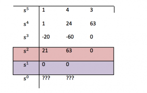
The row of zeros indicates that some of the roots of the characteristic equations are placed on the Imaginary Axis (case of Marginal Stability). Define Auxiliary Equation as an equation with coefficients from the Array row immediately above the row of zeros:
[latex]Q_{aux}(s) = 21s^{2} + 63[/latex]
Roots of Auxiliary Equations describe the system poles on Imaginary axis:
[latex]Q_{aux}(s) = 0[/latex]
[latex]s^{2} + 3 = 0[/latex]
[latex]s_{1} = j\sqrt{3} , s_{1} = -j\sqrt{3}[/latex]
Routh has proven that we can use the coefficients of a derivative of the auxiliary equation to complete the Routh Array:
[latex]Q_{aux}(s) = 21s^{2} + 63[/latex]
[latex]\frac{dQ_{aux}(s)}{ds} = 42s[/latex]
The fifth row, which was a row of zeros in the original Routh Array, is now replaced by:

The complete Routh Array is now as follows:

In this particular case looking at the first column, we can observe two sign changes (from +1 to -20 and from -20 to +21). This indicates that a) the system is unstable, and b) that it has two unstable poles (in RHP – the Right-Hand Part of the S-Plane).
| A quick check with MATLAB (“roots” command) shows that indeed the system has two unstable poles:
|
Two unstable poles: [latex]+1\pm j2.4495[/latex]
Also, observe the two poles on the Imaginary Axis are: [latex]\pm j\sqrt{3}[/latex], as calculated from the Auxilliary Equation. |

Auxiliary Equation is an extremely important concept because it enables us to determine stable ranges of Proportional Gains that can be safely used in a closed loop system.
| NOTE – for one possible application of the Auxilliary Equation, refer to your Lab # 1. |
2.3.4 Examples
2.3.4.1 Example
Use the Routh-Hurwitz Criterion of Stability on a system with the following Characteristic Equation [latex]Q(s)[/latex]:
[latex]Q(s) = s^{3} + s^{2} + 2s + 8 = 0[/latex]
2.3.4.2 Example
Use the Routh-Hurwitz Criterion of Stability on a system with the following Characteristic Equation [latex]Q(s)[/latex]:
[latex]Q(s) = s^{4} + s^{3} + 3s^{2} + 5s + 10 = 0[/latex]
