2.6 Examples

2.6.1 Example

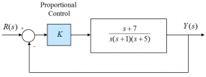
Consider a closed loop system as shown. Determine the range of stable operations for the Proportional Controller with the gain K.

2.6.2 Example

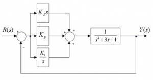
Consider the block diagram shown below, describing a process under the so-called Proportional-Integral-Derivative (PID) Control, as shown in the following Figure. Is the system open loop stable? Justify your answer. Next, let the Integral Gain [latex]K_{i}=10[/latex] and use the Routh-Hurwitz criterion to find the range of Derivative Gains [latex]K_{d}[/latex] and Proportional Gains [latex]K_{p}[/latex] in terms of [latex]K_{i}[/latex], so that the closed loop stability is achieved.

2.6.3 Example

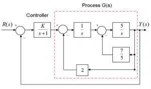
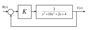
Consider the block diagram shown below and simplify it to find first the open loop, then the closed loop system transfer function as a function of gain K. Is the open loop system stable? Next, establish the range of gains K for a stable closed loop operation of this system. Find the critical value of the gain, at which the system would be marginally stable, and the corresponding frequency of oscillations of the marginally stable response, [latex]\omega_{osc}[/latex].

2.6.4 Example

Consider a unit feedback system under Proportional Control, as shown:

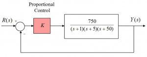
Apply the Routh-Hurwitz stability criterion to this system and determine the critical value(s) of gain, [latex]K_{crit}[/latex], for system stability, as well as the frequency of oscillations,[latex]\omega_{osc}[/latex], resulting when [latex]k=K_{crit}[/latex].

Next, assuming that the operational values of the proportional gain are again, [latex]K_{op}= 1[/latex] and [latex]K_{op}= 10[/latex], compute the corresponding values of the Gain Margins.

2.6.5 Example

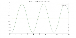
Part 1: Consider the SIMULINK diagram representing a certain closed loop system under Proportional Control:

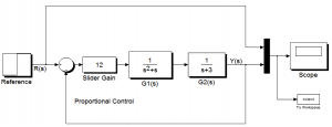
When the gain value is as indicated in the diagram, the “Scope” graph is as shown on the next page. What is the frequency of oscillations of the system response, [latex]\omega_{osc}[/latex]?

Part 2: Assume that the constant Proportional Gain block (Slider Gain) in the SIMULINK diagram is replaced with a variable Proportional Gain K, and use theory you have learned to find the range of the Proportional Gain values for the stable system operation. Determine the critical value of the Proportional Gain, [latex]K_{crit}[/latex], for which the system becomes marginally stable – how does it compare with the information provided by SIMULINK?

Assuming that the operational gain of the system [latex]K_{op}= 1[/latex], what is the system Gain Margin? Repeat for [latex]K_{op}= 3[/latex].

2.6.6 Example

Consider four control systems, each with a characteristic equation as shown below. Which system is stable?

System 1: [latex]s^{4}+ 4s^{2}+ 12s +6 = 0[/latex]

System 2: [latex]s^{4} - 3s^{3} +2s^{2}+ 12s+ 6 = 0[/latex]

System 3: [latex]s^{4}+ 3s^{3} +2s^{2} - 6 = 0[/latex]

System 4: [latex]s^{4} +3s^{3} +4s^{2}+ 1s +1 = 0[/latex]

2.6.7 Example

Consider the following closed loop control system under the so-called Proportional Control (P), where the system parameters are as follows: [latex]a=1, b=8, c=7[/latex].

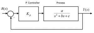
Find the closed loop transfer function of this system in terms of the Proportional Controller gain, [latex]K_{p}[/latex]. Find the condition for the gain [latex]K_{p}[/latex] so that the closed loop operation of the system is stable, and determine the practical range of [latex]K_{p}[/latex] values for the stable closed loop operation of the system.

What is the critical value of the Proportional Controller gain, [latex]K_{crit}[/latex] , that will cause the closed loop system to be marginally stable? When the gain is set at this critical value, [latex]K_{p} = K_{crit}[/latex] , what will the resulting frequency of oscillations, [latex]\omega_{osc}[/latex], be (in radians/sec)?

2.6.8 Example

Consider the following closed loop control system under the so-called Proportional Integral Control (P I), where the system parameters are the same as in Example 2.6.7:  [latex]a=1, b=8, c=7[/latex].

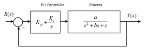
Find the closed loop transfer function of this system in terms of both Proportional and Integral Controller gains, [latex]K_{p}[/latex] and [latex]K_{i}[/latex]. Find the condition in terms of gains [latex]K_{p}[/latex] and [latex]K_{i}[/latex] so that the closed loop operation of the system is stable, and determine the practical range of each gain, [latex]K_{p}[/latex] and [latex]K_{i}[/latex] required for the stable closed loop operation of the system;

Now, assume the proportional Controller gain value is [latex]K_{p} = 3[/latex]; what is the range for the Integral Controller gain, [latex]K_{i}[/latex], for the stable closed loop operation of the system? What is the critical value of the Integral Controller gain, [latex]K_{crit}[/latex], that will cause the closed loop system to be marginally stable? When the Integral Controller Gain is set at this critical value, [latex]K_{i} = K_{crit}[/latex] , what will the resulting frequency of oscillations, [latex]\omega_{osc}[/latex], be (in radians/sec)?

2.6.9 Example

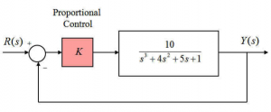
Consider the following closed loop control system under Proportional Control:

Find the closed loop transfer function of this system in terms of its Proportional Gain K. Find the practical range of Controller Gain values such that the closed loop operation of the system is stable. What is the critical value of the Proportional Gain, [latex]K_{crit}[/latex], that will cause the closed loop system to be marginally stable? When the Controller Gain is set at its critical value, [latex]K = K_{crit}[/latex], what will be the resulting frequency of oscillations, [latex]\omega_{osc}[/latex], (in radians/sec)? What will be the period of these oscillations, [latex]T_{period}[/latex]?

2.6.10 Example

Consider the following closed loop control system under the so-called Proportional Integral Control (P+I):

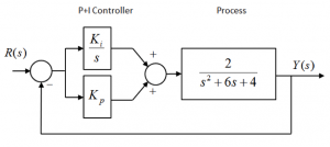
Find the closed loop transfer function of this system in terms of both Proportional and Integral Controller gains, [latex]K_{p}[/latex] and [latex]K_{i}[/latex]. Next, find the conditions in terms of gains [latex]K_{p}[/latex] and [latex]K_{i}[/latex] so that the closed loop operation of the system is stable, and determine the range of each gain, [latex]K_{p}[/latex] and [latex]K_{i}[/latex], required for such stable closed loop operation of the system.

Next, assume the Integral Controller gain value is [latex]K_{i}= 18[/latex]. Answer the following questions:

What is the range for the Proportional Controller gain, [latex]K_{p}[/latex] for the stable closed loop operation of the system? What is the critical value of the Proportional Controller gain, [latex]K_{crit}[/latex], that will cause the closed loop system to be marginally stable? When the Proportional Controller Gain is set at this critical value, [latex]K_{p} = K_{crit}[/latex], what will be the resulting period of oscillations, [latex]T_{period}[/latex], in seconds?

Finally, assume the Integral Controller gain value is [latex]K_{i}= 6[/latex] and the Proportional Controller gain, [latex]K_{p} = -0.5[/latex]. Answer the following questions:

Will the response be stable? What will be the steady state value of a response to a unit reference? Is this a good Proportional Controller Gain value to operate the system with? If yes, briefly explain why. If not, briefly explain why.

2.6.11 Example

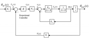
Consider the servo-control system for a position control of one of the joints of a robot arm, operating under Proportional Control (controller gain [latex]K[/latex]), as shown in the following Figure.[latex]\Theta_{ref}[/latex] is the reference angular position signal, [latex]\Theta_{load}[/latex] is the actual angular output shaft position signal, [latex]V_{a}[/latex] is the armature voltage, [latex]T_{m}[/latex] is motor torque and [latex]\Omega[/latex]is shaft velocity. This control system utilizes an armature-controlled DC motor, with an analog rotary position sensor.

The systems parameters are as follows: [latex]K_{t} = 0.1\frac{V}{rad}[/latex]– transducer gain of the sensor, [latex]K_{a} = 50\frac{V}{V}[/latex] – amplifier gain, [latex]K_{m} = 2\frac{N\cdot m}{A}[/latex]– motor torque constant,[latex]R = 2.0\Omega[/latex] – armature resistance, [latex]L = 0.1H[/latex] – armature inductance, [latex]K_{b} = 2\frac{V\cdot sec}{rad}[/latex]– CEMF constant, [latex]J = 0.5\frac{N\cdot m\cdot sec^{2}}{rad}[/latex]– motor & load (robot arm) inertia, and [latex]B = 0.7\frac{N\cdot m\cdot sec}{rad}[/latex]   is the motor & load linear friction coefficient.

Find the closed loop transfer function between the reference angle [latex]\Theta_{ref}[/latex] and the load position angle. Next, find the critical value of the controller gain, [latex]K_{crit}[/latex], such that the closed loop system is marginally stable. Find the corresponding value of the resulting oscillations, [latex]\omega_{osc}[/latex], in rad/sec. Next, determine the practical range (or ranges) of the controller gain [latex]K[/latex], for a stable operation of the closed loop system.

2.6.12 Example

Consider a unit feedback system under Proportional Control, [latex]K[/latex]. The process transfer function [latex]G(s)[/latex] is described as follows:

[latex]G(s) =\frac{3000}{(s 1)(s 10)(s 20)}[/latex]

What is the critical gain, [latex]K_{crit}[/latex], at which the system will be marginally stable? What is the frequency of oscillations, [latex]\omega_{osc}[/latex], at that gain?

2.6.13 Example

Consider a unit feedback system under Proportional Control, as shown:

Find the closed loop transfer function of this system with [latex]K[/latex] as its parameter and determine the system characteristic equation. Determine the range of values of the Proportional Gain [latex]K[/latex] so that the system response remains stable, and the critical value of the gain, [latex]K_{crit}[/latex], for which the system becomes marginally stable. What is the frequency of oscillations, [latex]\omega_{osc}[/latex], of the system response when the system becomes marginally stable?

2.6.14 Example

Consider a unit feedback system operating under Proportional Control (Controller Gain is [latex]K_{p}[/latex], where the process transfer function is described as follows:

[latex]G(s) = \frac{(s 10)^{2}}{(s 1)^{3}}[/latex]

Find the closed loop transfer function of this system and the critical value (or values) of the controller gain, [latex]K_{crit}[/latex], such that the closed loop system is marginally stable. Find the corresponding value (or values) of the resulting oscillations, [latex]\omega_{osc}[/latex], in rad/sec. Next, determine the practical range (or ranges) of the controller gain, [latex]K_{p}[/latex], for a stable operation of the closed loop system.