
Chapter 12
12.2 Model from Open Loop Frequency Response
12.2.1 Phase Margin vs. Damping ratio
Consider again the closed-loop system in Figure 12‑1. The closed-loop transfer function is that of the standard 2nd order system with the DC gain equal to 1, shown in Equation 12‑1. The closed-loop system is type 1 – one integrator in G(s). Let us now consider the open-loop system frequency response of that system:
| [latex]G(j\omega)=\frac{\omega_n^2}{j\omega(j\omega+2\zeta\omega_n)}[/latex] |
Equation 12‑14 |
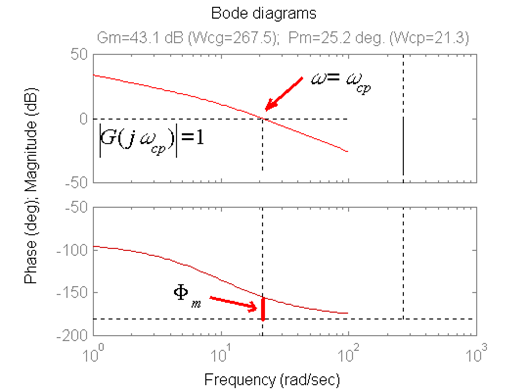
Let us find the system Phase Margin, [latex]\Phi _m[/latex], defined by Equation 11‑4. To find the frequency of crossover, the open-loop gain in Equation 12‑15 is set to 1 (0dB), as per the definition of the Phase Margin, [latex]\Phi _m[/latex], shown in Figure 12‑8.
It will be shown that the Phase Margin,[latex]\Phi _m[/latex], relates to the closed-loop system transient performance (time-domain). This relationship forms the basis of the classical controller design in the frequency domain.
| [latex]\omega=\omega_{cp}[/latex] [latex]\left | G(j\omega_{cp}) \right |=1[/latex] |
Equation 12‑15 |
| [latex]\frac{\omega_{n}^2}{\omega_{cp}\sqrt{\omega_{cp}^2+4\zeta^2\omega_n^2}}=1[/latex] [latex]\omega_{n}^4=\omega_{cp}^2(\omega_{cp}^2+4\zeta^2\omega_n^2)[/latex] [latex]\omega_{cp}^4+4\zeta^2\omega_n^2\omega_{cp}^2-\omega_{n}^4=0[/latex] |
Equation 12‑16 |
The formula for a quadratic solution is applied:
| [latex]ax^4+bx^2+c=0[/latex] [latex]\Delta =b^2-4ac=[/latex] [latex]16\zeta^4\omega_{n}^4+4\omega_n^4=4\omega_n^4(4\zeta^4+1)[/latex] [latex]\sqrt{\Delta }=2\omega_n^2\sqrt{(4\zeta^4+1)}[/latex] [latex]x=\frac{-4\zeta^2\omega_n^2+2\omega_n^2\sqrt{(4\zeta^4+1)}}{2}=[/latex] [latex]-2\zeta^2\omega_n^2+\omega_n^2\sqrt{(4\zeta^4+1)}[/latex] [latex]\omega_{cp}^2=x=-2\zeta^2\omega_n^2+\omega_n^2\sqrt{(4\zeta^4+1)}[/latex] [latex]\left ( \frac{\omega_{cp}}{\omega_{n}} \right )^2= -2\zeta^2+\sqrt{(4\zeta^4+1)}[/latex] |
Equation 12‑17 |
Phase margin [latex]\Phi_m[/latex] can now be found:
| [latex]\Phi_m=180^{0}+\angle GH(\omega_{cp})=180^0-90^0-tan^{-1}\left ( \frac{\omega_{cp}}{2\zeta\omega_n} \right )[/latex] [latex]=90^0-tan^{-1}\left ( \frac{1}{2\zeta}\left ( \sqrt{-2\zeta^2+\sqrt{4\zeta^4+1}} \right ) \right )[/latex] [latex]tan(90^0-\alpha )=\frac{1}{tan \alpha}[/latex] [latex]tan(\Phi_m)=\frac{2\zeta }{\sqrt{-2\zeta^2+\sqrt{4\zeta^4+1}}}[/latex] [latex]\Phi_m=tan^{-1}\left ( \frac{2\zeta }{\sqrt{-2\zeta^2+\sqrt{4\zeta^4+1}}} \right )[/latex] |
Equation 12‑18 |
This relationship looks quite complicated, however, when plotted in Figure 12‑9, a very simple approximation becomes obvious:
| [latex]\Phi_m\approx 100.\zeta \mapsto \zeta \approx 0.01.\Phi_m[/latex] | Equation 12‑19 |
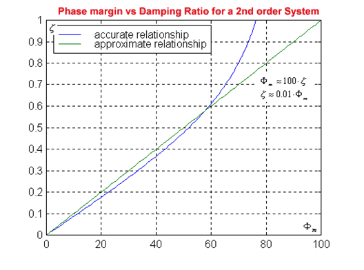
For Phase Margins between 0 and 15 degrees, and between 55 and 60 degrees, this approximation is very accurate. For Phase Margins between 15 and 55 degrees, as shown in Figure 12‑9, the actual value of the damping ratio is below the straight line approximation and Equation 12‑19 can be slightly modified:
| [latex]\Phi_m\approx 100.\zeta +5^0 \mapsto \zeta \approx 0.01.(\Phi_m-5^0)[/latex] | Equation 12‑20 |
