
Chapter 1
1.4 Laplace Transforms
Self-Study: Review your ELE532 Notes and other resources. You can also refer to the review material on the course website.
1.4.1 Definitions
|
[latex]F(s) = L[f(t)] = \int_{0}^{+\infty}f(t)e^{-st}dt[/latex] [latex]f(t) = L^{-1}[F(s)] = \frac{1}{2\pi j}\int_{\sigma - j\infty}^{\sigma + j\infty} F(s)e^{st}ds[/latex] |
Equation 1‑1 |
1.4.1.1 Final Value Theorem
| [latex]f_{ss} = \lim_{t\to\infty}f(t) = \lim_{s\to 0} sF(s)[/latex] | Equation 1‑2 |
1.4.1.2 Initial Value Theorem
| [latex]f_{0} = \lim_{t\to 0+}f(t) = \lim_{s\to\infty} sF(s)[/latex] | Equation 1‑3 |
1.4.1.3 Properties of Laplace transforms
| [latex]F(s)e^{-Ts}[/latex] | [latex]f(t-T)\cdot 1(t)[/latex] |
| [latex]F(s+a)[/latex] | [latex]f(t)e^{-at}\cdot 1(t)[/latex] |
| [latex]sF(s) - f(0+)[/latex] | [latex]\frac{df(t)}{dt}[/latex] |
| [latex]S^{2}F(s) - sf(0+) - \frac{df(0+)}{dt}[/latex] | [latex]\frac{d^{2}f(t)}{dt^{2}}[/latex] |
| [latex]\frac{1}{s}F(s)[/latex] | [latex]\int_{0+}^{+\infty}f(t)dt[/latex] |
| [latex]F_{1}(s)\cdot F_{2}(s)[/latex] | [latex]f_{1}(t)\ast f_{2}(t)[/latex] |
1.4.2 Solving for System Response
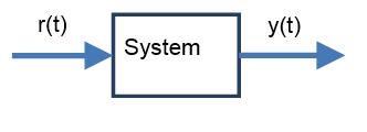
Parametric models cannot be developed without math. Laws of physics describe dynamic Linear Time-Invariant (LTI) systems using ordinary differential equations. To simplify their analysis, Laplace transform is used. Consider a certain LTI (Linear Time-Invariant), SISO (Single Input Single Output) system:
Let the input – output relationship for the system be described by the following nth order differential equation:
| [latex]\frac{d^{n}y}{dt^{n}}+a_{n-1}\frac{d^{n-1}y}{dt^{n-1}}+...+a_{1}\frac{dy}{dt} + a_{0}y = b_{m}\frac{d^{m}u}{dt^{m}} + b_{m-1}\frac{d^{m-1}u}{dt^{m-1}} + ...+ b_{1}\frac{du}{dt} + b_{0}u[/latex] | Equation 1‑4 |
The equation parameters relate to physical aspects of the system. The time domain description of systems is not convenient for quick paper-and-pencil speculations. To simplify math, Classical Control uses a Laplace Transform system description, which converts the differential equations into their algebraic equivalents in the s-domain. The solution for y(t) can then be found using inverse Laplace transformation to Y(s).
1.4.3 Two Transfer Functions Models: TF and ZPK
In the transform domain, the input-output relationship of the system is defined by a transfer function G(s), defined as a ratio of the Laplace transform of the system output signal y(t), to the Laplace transform of the system input signal u(t), with any initial conditions in the system set to zero. The system transfer function G(s) can be thought of as a dynamic gain of the system:
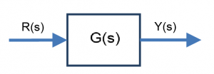
Block diagrams are used to graphically represent systems and their components, as shown above. In order to find G(s), a Laplace transform of the system differential equation in Equation 1‑4 is taken:
| [latex]s^{n}Y(s) + a_{n-1}s^{n-1}Y(s) + ... + a_{1}sY(s) + a_{0}Y(s) = b_{m}s^{m}U(s) + b_{m-1}s^{m-1}U(s) + ... + b_{1}sU(s) + b_{0}U(s)[/latex]
[latex]G(s) = \frac{Y(s)}{U(s)} = \frac{b_{m}s^{m} + b_{m-1}s^{m-1} + ... + b_{1}s + b_{0}}{s^{n} + a_{n-1}s^{n-1} + ... + a_{1}s + a_{0}}[/latex] |
Equation 1‑5 |
Transfer functions are ratios of polynomials written in terms of the s-operator. The resulting function in Equation 1‑5 is a ratio of two polynomials, N(s) and D(s):
| [latex]G(s) = \frac{N(s)}{D(s)} = \frac{b_{m}s^{m} + b_{m-1}s^{m-1} + ... + b_{1}s + b_{0}}{s^{n} + a_{n-1}s^{n-1} + ... + a_{1}s + a_{0}}[/latex] |
Equation 1‑6 |
Roots of the numerator polynomial of G(s) in Equation 1‑6 are called system zeros, [latex]z_{i}[/latex], and roots of the denominator polynomial are called system poles, [latex]p_{i}[/latex].
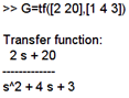
[latex]G(s) = \frac{Y(s)}{U(s)} = \frac{2s + 20}{s^{2} + 4s + 3}[/latex]
The same transfer function [latex]G(s)[/latex] can be represented in the so-called ZPK form (factorized form):
| [latex]G(s) = \frac{K\prod_{i}^{m}(s-z_{i})}{\prod_{j}^{n}(s-p_{j})}[/latex] |
Equation 1‑7 |
K is a multiplier. It is important to see the difference between K and Kdc, which denotes the DC gain of the system (i.e. s=0):
| [latex]K_{dc} = G(0) = \frac{N(0)}{D(0)} = \frac{b_{0}}{a_{0}} = \frac{K\prod_{i}^{m}(-z_{i})}{\prod_{j}^{n}(-p_{j})}[/latex] |
Equation 1‑8 |
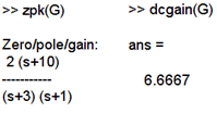
Our transfer function can be factorized and the multiplier gain K is equal to 2:
| [latex]G(s) =\frac{Y(s)}{U(s)} = \frac{2(s+10)}{(s+1)(s+3)}[/latex] |
The DC gain of our transfer function is:
| [latex]K_{DC} = G(0) = \frac{2(10)}{(1)(3)} = 6.667[/latex] |
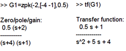
In MATLAB the transfer function can be shown in a factorized form by using the “zpk” command, and the DC gain can be found using “dcgain” command:
Locations of the system poles and zeros can be presented graphically as the so-called Pole-Zero Map.
1.4.4 Partial Fractions Technique
If a certain control system is described by a transfer function G(s), the system response can be found as [latex]Y(s) = U(s) \cdot G(s)[/latex]. Since Laplace Transform Tables do not provide exhaustive solutions, a technique of a Partial Fractions Expansion is used to find inverse Laplace Transforms for various time functions – see a table of basic Laplace – Time Domain Function pair shown in Table 1‑2.
1.4.4.1 Residues – Distinct Roots Case
| [latex]Y(s) = \frac{N(s)}{\prod_{i}^{n}(s-p_{i})} = \frac{N(s)}{D(s)}[/latex] [latex]Y(s) = \frac{K_{1}}{s-p_{1}} +\frac{K_{2}}{s-p_{2}} + ... + \frac{K_{n}}{s-p_{n}}[/latex] |
Equation 1‑9 |
| [latex]K_{1} = \frac{N(s)(s-p_{1})}{D(s)}\vert_{s=p_{1}}[/latex] [latex]K_{2} = \frac{N(s)(s-p_{2})}{D(s)}\vert_{s=p_{2}}[/latex] [latex]\vdots[/latex] [latex]K_{n} = \frac{N(s)(s-p_{n})}{D(s)}\vert_{s=p_{n}}[/latex] |
Equation 1‑10 |
1.4.4.2 Residues – Multiple Roots Case
This is the case for Laplace Transforms with multiple powers of some roots. Assume multiplicity of m for root [latex]r_{1}[/latex]:
| [latex]Y(s) = \frac{N(s)}{\prod_{i}^{n} (s-p_{i})} = \frac{N(s)}{D(s)}[/latex] [latex]Y(s) = \frac{K_{1}}{s-r_{1}} + \frac{K_{2}}{(s-r_{1})^2} + ... + \frac{K_{m}}{(s-r_{1})^{m}} + ... + \frac{K_{n}}{s-p_{n}}[/latex] |
Equation 1‑11 |
Residues for distinct roots calculated as before:
| [latex]K_{m+1} = \frac{N(s)(s-p_{1})}{D(s)}\vert_{s = p_{m+1}}[/latex] [latex]\vdots[/latex] [latex]K_{n} = \frac{N(s)(s-p_{n})}{D(s)}\vert_{s = p_{n}}[/latex] |
Equation 1‑12 |
To calculate residues for a multiple root, multiply both sides of Equation 1‑12 by [latex](s-r_{1})^{m}[/latex]and substitute the value of the root [latex]r_{1}[/latex]:
| [latex]\frac{N(s)}{D(s)} = \frac{K_{1}}{s-r_{1}} + \frac{K_{2}}{(s-r_{1})^{2}} + ... + \frac{K_{m}}{(s-r_{1})^{m}} + ... + \frac{K_{n}}{s-p_{n}}[/latex] [latex]\frac{N(s)(s-r_{1})^{m}}{D(s)} = \frac{K_{1}(s-r_{1})^{m}}{s-r_{1}} + \frac{K_{2}(s-r_{1})^{m}}{(s-r_{1})^{2}} + ... + K_{m} + ... + \frac{K_{n}(s-r_{1})^{m}}{s-p_{n}}[/latex] [latex]\frac{N(s)(s-r_{1})^{m}}{D(S)}\vert_{s=r_{1}} = K_{m}[/latex] |
Equation 1‑13 |
To calculate the residues for the second multiplicity of the root [latex]r_{1}[/latex]:
| [latex]\frac{d}{ds}\left(\frac{N(s)(s-r_{1})^{m}}{D(s)}\right) = \frac{d}{ds}\left( \frac{K_{1}(s-r_{1})^{m}}{s-r_{1}} + \frac{K_{2}(s-r_{1})^{m}}{(s-r_{1})^{2}} + ... + K_{m} + ... + \frac{K_{n}(s-r_{1})^{m}}{s-p_{n}}\right)[/latex] [latex]\frac{d}{ds}\left(\frac{N(s)(s-r_{1})^{m}}{D(s)}\right)\vert_{s=r_{1}} = 0 + ... + K_{m-1} + 0 + ... + 0[/latex] |
Equation 1‑14 |
| Laplace Transform | Time Domain Function |
| [latex]1[/latex] | [latex]\sigma (t)[/latex] |
| [latex]\frac{1}{s}[/latex] | [latex]1(t)[/latex] |
| [latex]\frac{1}{s^{2}}[/latex] | [latex]t \cdot 1(t)[/latex] |
| [latex]\frac{1}{s^{k+1}}[/latex] | [latex]\frac{t^{k}}{k!}1(t)[/latex] |
| [latex]\frac{1}{s+a}[/latex] | [latex]e^{-at} \cdot 1(t)[/latex] |
| [latex]\frac{1}{(s+a)^{2}}[/latex] | [latex]te^{-at} \cdot 1(t)[/latex] |
| [latex]\frac{a}{s(s+a)}[/latex] | [latex](1-e^{-at})\cdot (t)[/latex] |
| [latex]\frac{a}{s^{2}+a^{2}}[/latex] | [latex]sin(at)\cdot 1(t)[/latex] |
| [latex]\frac{s}{s^{2}+a^{2}}[/latex] | [latex]cos(at)\cdot 1(t)[/latex] |
| [latex]\frac{s+a}{(s+a)^{2} + b^{2}}[/latex] | [latex]e^{-at}\cdot cos(bt)\cdot 1(t)[/latex] |
| [latex]\frac{b}{(s+a)^{2} + b^{2}}[/latex] | [latex]e^{-at}\cdot sin(bt)\cdot 1(t)[/latex] |
| [latex]\frac{a^{2} + b^{2}}{s[(s+a)^{2} + b^{2}]}[/latex] | [latex]\left (1-e^{-at}\cdot (cos(bt) + \frac{a}{b}\cdot sin(bt))\right )\cdot 1(t)[/latex] |
| [latex]\frac{\omega_{n}^{2}}{s^{2} + 2\zeta\omega_{n}s +\omega_{n}^{2}}[/latex] | [latex]\frac{\omega_{n}}{\sqrt{1-\zeta^{2}}}e^{-\zeta\omega_{n}t} \cdot sin \left(\omega_{n} \sqrt{1-\zeta^{2}t} \right)\cdot 1(t)[/latex] |
| [latex]\frac{\omega_{n}^{2}}{s(s^{2} + 2\zeta\omega_{n}s +\omega_{n}^{2})}[/latex] | [latex]\left( 1 - \frac{1}{\sqrt{1-\zeta^{2}}}e^{-\zeta\omega_{n}t} \cdot sin \left(\omega_{n} \sqrt{1-\zeta^{2}} t+ cos^{-1}(\zeta)\right) \right) \cdot 1(t)[/latex] |
To calculate the residues for the remaining multiplicities of the root r1, use this recursive formula:
| [latex]\frac{1}{2!}\frac{d^{2}}{ds^{2}} \left( \frac{N(s)(s-r_{1})^{m}}{D(s)} \right) \vert_{s = r_{1}} = K_{m-2}[/latex] [latex]\frac{1}{(m-1)!}\frac{d^{m-1}}{ds^{m-1}} \left( \frac{N(s)(s-r_{1})^{m}}{D(s)}\right)\vert_{s = r_{1}} = K_{m}[/latex] |
Equation 1‑15 |
1.4.5 Examples
1.4.5.1 Example
Consider a system described by the following transfer function and find the pole-zero model of the transfer function and its DC gain.
[latex]G(s) = \frac{2s+3}{S^{2}+3s+2}[/latex]
HINT: Use MATLAB software to check your results in this, and the remaining examples in this section.
1.4.5.2 Example
Consider a system described by the following transfer function:
![]()
[latex]\frac{5s^{3} + 30s^{2} +55s + 30}{s^{5} + 14s^{4} + 62s^{3} + 110s^{2} + 153s + 140}[/latex]
Find the pole-zero model of the transfer function and its DC gain. HINT: Use Matlab.
1.4.5.3 Example
A certain LTI system is described as having one zero and four poles, as follows:
[latex]z_{1} = -2.2[/latex],
[latex]p_{1} = -1 + j1[/latex],
[latex]p_{2} = -1 - j1[/latex],
[latex]p_{3} = -10[/latex],
[latex]p_{4} = -2[/latex],
It is also recorded that the system has a DC gain of 5.
Write the complete transfer function of the system in a ZPK form.
1.4.5.4 Example
Consider a system described by the following transfer function:
[latex]G(s) = \frac{10s^{2} + 30s + 20}{s^{4} + 14s^{3} + 68s^{2} + 130s + 75}[/latex]
Create an LTI object representing this system using both the transfer function model and the zero-pole-gain model. Extract zero-pole-gain data and numerator-denominator from the LTI object. Obtain the system dc gain and the pole-zero map of the transfer function. Obtain a minimum realization of this system. Use MATLAB to solve this problem.
1.4.5.5 Example
Consider a system described by the following transfer function:
[latex]G(s) = \frac{Y(s)}{U(s)} = \frac{s^{2} + 3s + 3}{s^{3} + 6s^{2} + 11s + 6}[/latex]
Find an analytical expression for an impulse response of the system.
1.4.5.6 Example
A certain control system is described by the following transfer function:
[latex]G(s) = \frac{Y(s)}{U(s)} = \frac{2s+8}{s^{3} + 5s^{2} + 8s + 4}[/latex]
Find an analytical expression for a step response of the system.
1.4.5.7 Example
A certain control system is described by the following closed loop transfer function:
[latex]G_{cl}(s) = \frac{45(s+6)}{(s^{2} + 65s + 354)s}[/latex]
Find an analytical expression for a step response of the system – note the integrator term in the denominator!
1.4.5.8 Example
A certain control system is described by the following closed loop transfer function:
[latex]G_{cl}(s) = \frac{45(s+6)}{s^{3} + 20s^{2} + 129s + 270}[/latex]
One of the closed loop poles is at -5. Find an analytical expression for a step response of the system.
