1.6 Basic Block Diagrams

1.6.1 Blocks in Series

Consider two cascade blocks as shown in Figure 1‑17. What is the transfer function relating signals [latex]Y(s)[/latex] and [latex]R(s)[/latex]?

[latex]X(s) = R(s) \cdot G_{1}(s)[/latex],         [latex]Y(s) = R(s) \cdot G_{1}(s) \cdot G_{2}(s)[/latex]

[latex]Y(s) = X(s) \cdot G_{2}(s)[/latex]          [latex]G(s) = \frac{Y(s)}{R(s)} = G_{1}(s)\cdot G_{2}(s)[/latex]

1.6.2 Blocks in Parallel

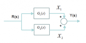
Consider two blocks in parallel as shown in Figure 1‑18. What is the transfer function relating signals [latex]Y(s)[/latex] and [latex]R(s)[/latex]?

[latex]X_{1}(s) = R(s) \cdot G_{1}(s)[/latex]

[latex]X_{2}(s) = R(s) \cdot G_{2}(s)[/latex]

[latex]Y(s) = X_{1}(s) + X_{2}(s)[/latex]

[latex]G(s) = \frac{Y(s)}{R(s)} = \frac{R(s) \cdot G_{1}(s) + R(s) \cdot G_{2}(s)}{R(s)} = G_{1}(s) + G_{2}(s)[/latex]

1.6.3 Basic Closed Loop Revisited 

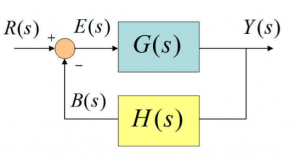
Consider the basic closed loop system identical to the one shown in Chapter 1.2.2, but this time with the static block gains replaced by their dynamic equivalents, i.e. their transfer functions describing a relationship of time domain signals as represented in Laplace Transform domain. Let us derive the closed loop transfer function relating system output to the reference.

[latex]Y(s) = E(s) \cdot G(s)[/latex]

[latex]E(s) = R(s) - B(s)[/latex]

[latex]B(s) = Y(s) \cdot H(s)[/latex]

[latex]G_{cl}(s) = \frac{Y(s)}{R(s)} = ?[/latex]

Closed loop characteristic equation is then described as follows: