Chapter 14
14.3 Solved Examples for Polar Plots
14.3.1 Example
Consider the following transfer function:
[latex]G(s) = \frac{200}{s^3+11s^2+38s+4}[/latex]
Consider its frequency response, [latex]G(j \omega )[/latex], at a specific frequency of [latex]\omega =1[/latex] rad/sec. Show its rectangular and polar forms.
[latex]G(j \omega )= \frac{200}{(j \omega )^3 +11(j \omega )^2 +38(j \omega )+4}[/latex]
[latex]= \frac{200}{-j( \omega )^3 -11( \omega )^2 +38(j \omega )+4}=[/latex] [latex]\frac{200}{(4-11 \omega^2 )+j \omega (38- \omega^2 )}[/latex]
[latex]G(j1)= \frac{200}{-7+j37} =[/latex] [latex]\frac{200(-7-j37)}{49+1369} =-0.9873-j5.2186[/latex]
The polar form of this function is:
[latex]\mid G(j1) \mid = \sqrt{(-0.9873)^2+(-5.2186)^2}=5.3112[/latex]
[latex]\angle G(j1) =-1.7578rad=-100.71 ^\circ[/latex]
[latex]G(j \omega )= \mid G(j \omega ) \mid \cdot e^{(j \angle G( \omega )}[/latex]
[latex]G(j1)=5.3112 \cdot e^{-j1.7578}[/latex]
[latex]G(j1) = 5.3112 \cdot e^{-j1.7578}=-0.9873-j5.2186[/latex]
14.3.2 Example
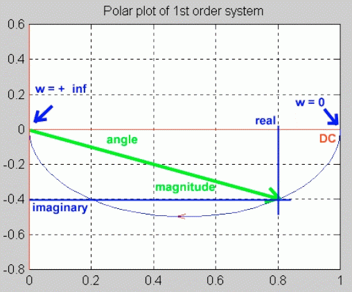
Consider a simple first order system, with one real pole:
[latex]G(s) = \frac{1}{10s+1}[/latex]
[latex]G(j \omega )=[/latex] [latex]\frac{1}{10j \omega +1} =[/latex] [latex]\frac{1}{ \sqrt{(10 \omega )^2+1} } \angle -tan^{-1}(10 \omega )[/latex]
[latex]M(j \omega )= \frac{1}{ \sqrt{(10 \omega )^2 +1} }[/latex]
[latex]\Phi (j \omega )= -tan^{-1}(10 \omega )[/latex]
Now consider the rectangular representation of the same frequency response function [latex]G(j \omega )[/latex]:
[latex]G(j \omega )= \frac{1}{1+10j \omega )} = \frac{1(1-10j \omega )}{ (1+10j \omega)(1-10j \omega)} = \frac{1}{1+100 \omega^2 }-j \frac{10 \omega }{1+100 \omega^2 }[/latex]
[latex]Re( \omega ) = \frac{1}{1+100 \omega^2 }[/latex]
[latex]Im( \omega )=- \frac{10 \omega }{1+100 \omega^2 }[/latex]
The standard frequency response plot (Bode Plot) with magnitude in decibels and phase in degrees is shown below. For the Polar Plot, crossovers with the Imaginary and Real axes can be calculated analytically by setting first the Real, then the Imaginary part to zero, and solving for frequency. In this example:
[latex]Re( \omega )=0 \implies[/latex] [latex]\omega = \infty[/latex]
[latex]Im ( \infty )=0[/latex]
[latex]Im ( \infty )=0 \implies[/latex] [latex]\omega = 0,[/latex] [latex]\omega = \infty[/latex]
[latex]Re(0) =1[/latex]
[latex]Re(\infty)=0[/latex]
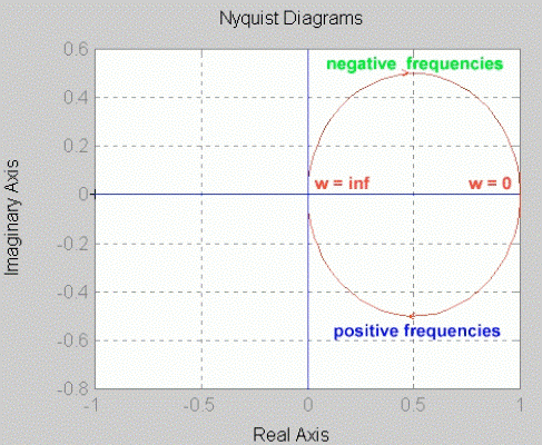
This indicates that the polar plot starts at (1, j0) location for [latex]\omega = 0[/latex] (DC condition), and ends at (0, j0) for [latex]\omega = \infty[/latex] . The sense of increasing frequency [latex]\omega[/latex] should always be shown on the polar plot. The polar plot of the system [latex]G(s)[/latex] is shown.
To do plot polar plots in MATLAB, use subroutine Nyquist – see below. The second plot (on the following page) shows a so-called Nyquist contour, which will be discussed in detail later. The Nyquist contour consists of the polar plot for positive frequencies,[latex]0 < \omega < + \infty[/latex], and its mirror image for negative frequencies, [latex]- \infty < \omega < 0[/latex].
14.3.3 Example
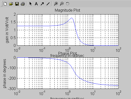
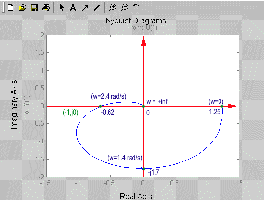
A process transfer function is described as follows: [latex]G(s) = \frac{10}{s^3+4s^2+6s+8}.[/latex] Frequency plots of [latex]G(s)[/latex] are shown. Sketch a polar plot for [latex]G(s)[/latex].
Solution: It is helpful to construct a table with the important coordinates:
| Frequency | Phase | Magnitude |
| [latex]\omega = 0[/latex] rad/s | [latex]\phi = 0 ^ \circ[/latex] | [latex]1.25[/latex] |
| [latex]\omega = 1.4[/latex] rad/s | [latex]\phi = -90 ^ \circ[/latex] | [latex]1.77[/latex] |
| [latex]\omega = 2.4[/latex] rad/s | [latex]\phi = -180 ^ \circ[/latex] | [latex]0.625[/latex] |
| [latex]\omega = + \infty[/latex] rad/s | [latex]\phi = -270 ^ \circ[/latex] | [latex]0[/latex] |
The resulting polar plot can be also plotted using MATLAB subroutine Nyquist.
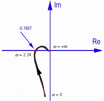
14.3.4 Example
Consider a unity feedback control system under Proportional Control. The process transfer function is described as follows:
[latex]G(s) = \frac{5}{s(s+1)(s+5)}[/latex]
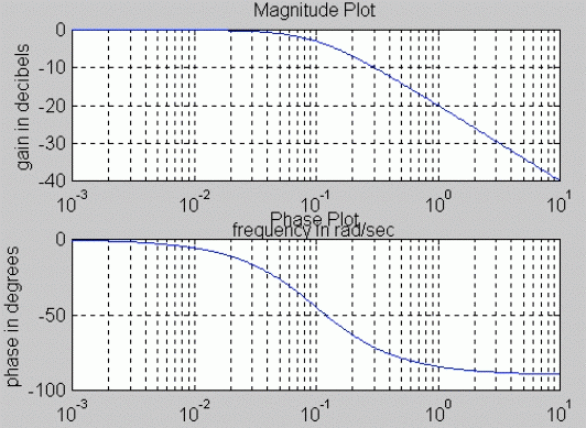
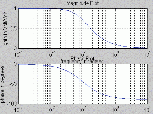
Frequency plots of [latex]G(s)[/latex] are shown. It is helpful to construct a table with the important coordinates read off the plot. Note that this is a Type I system, with an integrator, and therefore its polar plot will begin with an infinite gain at the DC level.
| Frequency | Phase | Magnitude in dB | Magnitude in Volt/Volt |
| [latex]\omega = 0[/latex]rad/s | [latex]\phi = -90 ^ \circ[/latex] | [latex]+ \infty[/latex] | [latex]+ \infty[/latex] |
| [latex]\omega = 224[/latex]rad/s | [latex]\phi = -180 ^ \circ[/latex] | [latex]-15.56[/latex] dB | [latex]0.1667[/latex] Volt/Volt |
| [latex]\omega = + \infty[/latex]rad/s | [latex]\phi = -270 ^ \circ[/latex] | [latex]- \infty[/latex] | [latex]0[/latex] |
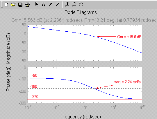
The resulting polar plot is shown.