8.3 Dominant System Dynamics and Reduced Order Models – Part 2

Responses of many industrial systems, even of a relatively higher order (which may be a result of linearization of the transportational delay), exhibit closed loop responses similar to the systems we discussed in Chapter 6.1 (first order systems) and Chapter 7.1 (second order underdamped systems), or, less frequently, in Chapter 6.2 (second order overdamped systems). This may be because system parameters have such values that pole-zero cancellations or near cancellations occur.

Or it may be because the system has some dominant dynamics – where several poles and zeros of the system have a much larger effect on the system response – we say they “dominate it” – than other poles and zeros. By ignoring the insignificant poles and zeros we can derive a reduced order model for the system behaviour.

One of your Computer Assignments deals with finding appropriate reduced order models to adequately represent system dynamic responses. Recall that a real pole (i.e. located on the Real axis) will result in a transient response that is an exponential where what we call the decay ratio is equal to the absolute value of the pole coordinate on the Real axis and is an inverse of the so-called time constant – see Equation 6‑2:

[latex]G(s) = \frac{K}{(s+p)} = \frac{K_{dc}}{(\tau s + 1)}[/latex]

[latex]y_{step}(t) = \frac{k}{a} \cdot\big( 1-e^{pt} \big) \cdot 1(t) = K_{dc} \Bigg( 1-e^{-\frac{t}{\tau}}  \Bigg) \cdot 1(t)[/latex]

[latex]\sigma = p = \frac{1}{\tau}[/latex]

Also recall that a pair of complex poles (i.e. located away from the Real axis) will result in a transient response that is an oscillation with an exponential envelope where the decay ratio is equal to the absolute value of the real coordinate of the poles and is an inverse of the so-called time constant – see Figure 7‑2 and Equation 7‑5:

[latex]G_{m}(s) = K_{dc} \frac{\omega_{n}^{2}}{s^{2}+2\zeta\omega_{n}s + \omega_{n}^{2}}[/latex]

[latex]y_{step}(t) = K_{dc} \cdot \Bigg( 1 - \frac{e^{-\zeta\omega_{n}t}}{\sqrt{1-\zeta^{2}}}sin\bigg(\omega_{n}\sqrt{1-\zeta^{2}t} + cos^{-1}\zeta \bigg) \Bigg)\cdot 1(t)[/latex]

[latex]\sigma = \zeta\omega_{n}[/latex]   [latex]\tau = \frac{1}{\sigma} = \frac{1}{\zeta\omega_{n}}[/latex]

Stable poles that are positioned close to the Imaginary axis will have short decay ratios , i.e. long time constants and will take a long time to settle, while poles far away in the LHP will have much larger decay ratios [latex]\sigma[/latex], i.e. much shorter time constants and will take a very short time to settle. Since the presence of such transients will only be felt at the very beginning of the step response, their effect on the time specs (i.e. Rise Time, Peak Time – where PO is measured, and Settling Time) can be safely ignored.

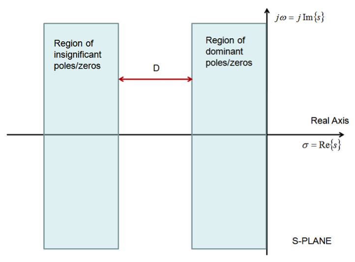
Figure 8‑1 shows the regions of dominant vs. insignificant system dynamics. Poles very far away in the LHP will be “insignificant” while those very close to the Imaginary axis will be “dominant”.

Of course, the question is – how do we decide the cut-off? The distance D separating the two regions shown in Figure 8‑1 is subject to discussion and may change depending on how tolerant our analysis/design is of inaccuracies. The generally accepted rule is that D should be 6 to 10 times the magnitude of the dominant pole (or of the real part of the dominant pair, in case of the complex poles.

To summarize, the system response is a superposition of the transient components where the shapes of components are dictated by the location of dominant poles. Once the insignificant poles are discarded, we can build a reduced order model for the system, based only on the dynamics of the dominant poles. The simplest cases of the reduced order models are: one dominant real pole – the system can be modelled by a first order model where a first order model as in Equation 6‑1, and a pair of dominant complex conjugate poles – the system can be modelled by a second order underdamped model as in Equation 7‑1.

Classical Control takes a particular interest in the second order underdamped model – if a closed loop response of a certain control system can be modelled by it, we can derive, as we will see later in the course, some relatively simple but effective control algorithms that depend on the parameters of this basic model described by Equation 7‑1. Chapter 7 dealt in detail with the relationship between the model parameters ([latex]K_{dc}, \zeta, \omega_{n}[/latex]) and the quality of the system response (specifications such as PO, Settling Time, Rise Time and Errors). Later we will be able to tie these parameters to the controller design.