14.4 Gain and Phase Margins vs. Polar Plots

14.4.1 Example Gain Margin from Polar Plot

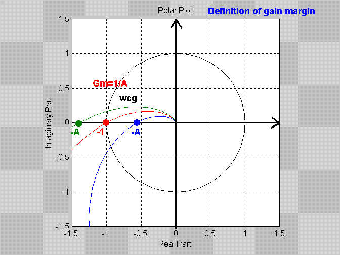
Let the crossover frequency be defined as [latex]\omega_{cg}[/latex], the frequency at which the phase plot crosses over the [latex]-180^ \circ[/latex] line. On the polar plot, this corresponds to the plot crossing the negative part of Real axis. Remember the definition of Gain Margin [latex]G_{m}[/latex] :

On the polar plot, Gain Margin [latex]G_m[/latex] can be found as an inverse of the coordinate A of the polar plot crossover with the Real axis, as shown next. If the crossover is to the right of (-1, j0) point,[latex]\mid A \mid < 1[/latex] ,[latex]G_{m}>1[/latex] , and the system is stable. If the crossover is to the left of (-1, j0) point,[latex]\mid A \mid>1[/latex] ,[latex]G_m[/latex] [latex]<1[/latex] , and the system is unstable.  

14.4.2 Example Phase Margin from Polar Plot

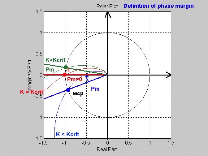
The crossover frequency defined as [latex]\omega_{cp}[/latex], is the frequency at which the polar plot crosses over the unit circle ([latex]0[/latex] dB = 1 Volt/Volt). Phase Margin [latex]\Phi_m[/latex] is defined as [latex]\Phi_m=180 ^ \circ + \angle GH( \omega_{cp} ).[/latex] Therefore, on the polar plot Phase Margin [latex]\Phi_m[/latex] can be found as the angle between the Real axis and the crossover of the polar plot with the unit circle, as shown in Error! Reference source not found. If this angle is above the Real axis, the system is unstable, if this angle is below the Real axis, the system is stable.

14.4.3 Solved Example

Consider a unit feedback closed loop system where the open loop transfer function [latex]G(s)[/latex] is known to be unstable and its transfer function [latex]G(s)[/latex] is known as [latex]G(s) = \frac{s+2}{s(s-2)} .[/latex] Such system can be stabilized by using an appropriately large value of the controller gain. We need to establish the critical gain [latex]K_{crit}[/latex] .

Solution Part 1: Let’s tackle this problem in s-domain. The system closed loop characteristic equation is:

[latex]1+KG(s)=0[/latex]

[latex]1+K \frac{s+2}{s(s-2)} =0[/latex]

[latex]s^2-2s+Ks+2K=0[/latex]

[latex]s^2+(K-2)s+2K=0[/latex]

For the 2^nd order system the necessary and sufficient condition of stability is that all coefficients of the characteristic polynomial are positive:

[latex]K-2>0[/latex]

[latex]K>0[/latex]

The critical value of the gain is [latex]K_{crit}=2[/latex] and the range of gains for stable system performance is:

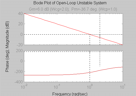
[latex]2

The frequency of oscillations [latex]\omega_{osc}[/latex] at the critical gain is equal to [latex]2[/latex] rad/s:

[latex]s^2+(K-2)s+2K=0[/latex]

[latex]K_{crit}=2[/latex]

[latex]s^2+4=0[/latex]

[latex]s= \pm j2[/latex]

[latex]\omega_{osc} =2[/latex]

The upper limit of the gain range will be determined by practical issues such as saturation.

Solution Part 2: Now let’s try to apply the Gain Margin and Phase Margin definitions to this system. The open loop frequency response has to be simulated as the system is open-loop unstable and no measurements on the open loop are possible. From the plot shown in Error! Reference source not found. we read:

[latex]G_m=+6dB=2[/latex]

[latex]\omega_{cg}=2[/latex]

The positive Gain Margin [latex]G_m= 6 dB = 2[/latex] Volt/Volt is measured at the crossover frequency [latex]\omega_{cp}[/latex] = 2 rad/s. This would have to be interpreted as the system being stable for gains lower than 2, which as we know from the s-domain analysis is not correct. On the other hand, the Phase Margin [latex]\Phi_m[/latex] is negative, indicating the system is unstable for gains [latex]< 2[/latex]. This is an example of when the Gain and Phase Margin definitions cannot be applied consistently to determine the system stability limits. A new, more general frequency domain based stability criterion will now be defined.